Territory of probability - page 8
You are missing trading opportunities:
- Free trading apps
- Over 8,000 signals for copying
- Economic news for exploring financial markets
Registration
Log in
You agree to website policy and terms of use
If you do not have an account, please register
The algorithm for winning a coin toss game is simple - if you get tails, bet on tails; if you get heads, bet on heads. If the number of flips is infinite, you win.)
Если монетка кривая, тогда матожидание будет положительным. Это алгоритм К. Шеннона. Если монетка идеальная, то хоть до потери пульса подбрасывай, матожидание будет нулевым, т.к. оно не зависит от количества испытаний.
Shannon is undoubtedly cool to get so many numbers in one place. ) It's easier with a coin. Tails and heads will form "streaks of heads" and "streaks of tails" if there are enough tosses. Each time betting on the previous side the player hopes to get into one of the tails stripes. Expectation equal to zero is not disputed. ) An infinite number of tosses allows the player to stop when he is in the plus enough for him.
If the game allows increasing/decreasing bets before each throw, a player may increase the bet after each win and decrease it after each loss. It seems to me that with such approach the expected payoff would be slightly above zero. As long as the initial capital is enough.)
bowie:
Shannon is undoubtedly cool to get so many numbers in one place. ) It's easier with a coin. If enough tosses are made, heads and tails will form "heads streaks" and "tails streaks". Each time betting on the previous side the player hopes to get into one of the tails stripes. Expectation equal to zero is not disputed. ) The infinite number of tosses allows the player to stop when he is in the plus enough for him.
If the game presupposes possibility to increase/decrease bets before each throw, a player may increase the bet after each win and decrease it after each loss. It seems to me that with such approach expectation of winning will be a bit higher than zero. As long as we have enough initial capital.
The probability that the player will sooner or later get the edge in his favor in case of a perfect coin is equal to 1, i.e., it is true according to the law of arcinus. Whether he has enough capital or not is another question. The law of arcinus says only that the capital at a constant bet is less than infinity, in order to get an edge.
A strip, i.e. continuous series of heads and tails does not contradict any theories, but advantages do not give either. If one is lucky, one will get a lucky streak. If you are unlucky, you will have bad luck. It has no effect on the mathematical expectation, but only on luck, i.e. the variance and the law of arcsinus.
The probability that a player will sooner or later get an advantage in the case of a perfect coin is 1, i.e. it is true according to the law of arcinus. Whether he has enough capital or not is another question. The law of arcinus only says that with a constant bet, you need less than infinity to get an edge.
And stripes, i.e. continuous series of heads and tails do not contradict any theories, but they do not give an advantage either. Whoever is lucky will get a lucky streak. If you are unlucky, you will have bad luck. It has no effect on the mathematical expectation, but only on luck, i.e. the variance and the law of arcsinus.
Reshetov, cut the crap! What does the law of arcinus have to do with it? The onset of outperformance in one's side does not mean that it will be sufficient to move into the positive yield zone, nor long enough to keep that yield in the positive zone.
You are both wrong. :)
In reality, all the coins are crooked. So Shannon's right. So am I. ;)
There is a script like this. And there are doubts about MathRand(). Who can say what? )
I propose to discuss here the methods and techniques of using probability theory to build trading systems. I will present my thoughts on this subject in the form of theses:
1) The probability of trend continuation in any part of it at any moment is higher than the probability of its reversal. Hence, the golden rule of trader: trade only with the trend.
2) The probability of winning with a random entry and the same TP and SL tends to 50% with increasing SL and TP.
3) The probability of winning when trading with a dynamic lot is lower than when trading with a fixed lot. I came to this conclusion on my own. I will try to prove it: let's say we have TS, which alternately triggered TP and SL, i.e. SL-TP-SL-TP-SL-TP, while SL = TP. Spread is not taken into account to ease understanding. When trading with a fixed lot, we obtain for example: -$10+$10-10$+$10-10$+$10$=0. When trading with dynamic lot we will get -10%+10%-10%+10%-10%+10%+10% and it will not lead us to zero profit, but will be a loss. For example, the deposit was 100, we got: 100-10%=90; 90+10%=99; 99-10%=89.1; 89.1+10%=98.01; 98.01-10%=88.209; 88.209+10%=97.0299, which was needed to prove, the loss is visible.
I am waiting for your comments and constructive criticism if anyone does not agree with my third thesis. If anyone has any other thoughts on the use of probability theory, please speak up.
I'll generalise a bit.
Suppose sl (loss) and tp(profit) are fixed in currency points.
Suppose we have a sufficiently large series of N trades.
N=N1+N2, where N1 - number of deals executed on tp, N2 - number of deals executed on sl.
Obviously, your trading system will be profitable if:
N1*tp - N2*sl >= spread * N
Do the maths - divide the left and right parts by N.
tp*N1/N - sl*N2/N >= spread
N1/N with the number of trades tending to infinity is nothing else but the probability of a profitable deal, let's call it p=N1/N
N2/N - then the probability of a losing trade, and will be equal to 1-p
We have:
p*tp - (1-p)*sl >=spread
Or another way:
p>=(sl + spread)/(sl+tp)
This p is what we create trading systems for. The probability that we want to increase. But you should always remember what it should be more than to be in profit.
For example, if you ignore the spread, and with equal tp and sl, your trading system will be profitable if p>0.5 ... etc.
If you make changes such as dynamic lot, things get much more complicated, and the probability of a profitable trade should be higher than in the above case.
I'm going to generalise a bit.
If we generalize a bit more and take into account the real situation 1) We MUST consider swaps 2) If we express SL and TP through spread in your formula, we get
p>= ( n_SL*spread + spread ) / (n_TP*spread + n_SL*spread) => p >= spread*(n_SL+1) / spread*(n_TP+n_SL) => p >= (n_SL+1)/(n_TP+n_SL)
If we draw it as a graph, we will see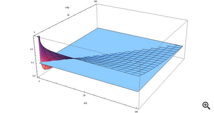
We see that with SL > TP our function is greater than 0.5, and the closer these values are...
Those, wishing to see for themselves - here is the formula in terms of the Wolfram-Alpha
An unexpected conclusion for many people, isn't it!)
I remember how long ago, here some people shouted - what I am saying here, that "SL is evil". :))
So now the young ones are here and they're more knowledgeable now. :)
Let's generalise a bit.
Let sl (loss) and tp(profit) be fixed in currency points.
...
If you make changes such as a dynamic lot then things get considerably more complicated and the probability of a profitable trade should be greater than in the above case.
As a purely theoretical formula it is of course interesting, but!!!
And if profit/loss is not fixed (but different for all trades), it will become even more complicated, and then we add floating spread to it - we will get such a mess that 10 EA developers will be spreading it all over the table for years.
This is why I tried to explain that it is difficult to make the market work with fixed take/loss values. By fixing the system developer clips the wings of the system (formally speaking, he does not make profit).
And tp and sl as fixed levels are only needed to protect the account from losses in case of a disconnection. But there are simpler solutions than fixing.
For example for real stops it's enough to set a two-way trawl moving stops behind the market and never triggers as long as there's a connection, and trade according to the situation.
This is my opinion.
You are both wrong :)
In reality, all coins are crooked. That's why Shannon's right. And me, too. ;)
In reality, coins change their curvature as they are tested.) Because you can't repeat the experiment under exactly the same conditions as the previous one. Random factors change and it may well be that their resulting curvature will be unbalanced for quite a long time. That is, it is a matter of the rate of change of the random factors relative to the experiment. How their internal time correlates with time between experiments.
Suppose for example a random process is generated based on a single sinusoid. If at the time of the experiment the value of the sine>0, then heads, less than that - tails. And then everything will depend on periodicity of our experiments, accuracy of time calculation and period of sine wave. If the intervals between experiments are not fixed and are much longer than the period of the sine wave, then the values will appear as random. If the time between experiments can be adjusted with an accuracy commensurate with the period of the sine wave, the series will be nonrandom - up to deterministic (depending on the accuracy of time measurement).
In general, random processes may not be periodic, but the cyclicality of them and the sum of all random factors must be present. For example, there cannot be a continuously increasing function instead of a sinusoid - then the resulting series will have an upward trend. Random processes affecting the series are in fact all non-random)))) just there is no information to accurately measure their phase at the time of the experiment, or there is insufficient precision of measurement.
If the sum of "random" factors is balanced in relation to 0 (as in the example with sine wave) - i.e. if it is above 0 and below 0, then the series under the influence of these factors will have mo = 0. If the sum is above 0 for a longer time, there will be a skew in favor of heads or in favor of tails. I.e. the sum of random factors is in some sense balanced and cyclic. We just don't know its exact value at the time of the experiment.
But the reality is complicated by the fact that the random factors can change and so can their sum. First it was a sine wave)) then it became a straight line at an angle if in those analogies. That's why the task of trading is to catch such moments when the series has a trend component going up or down. This requires the correspondence with the underlying processes. Return processes like a sinusoid form return patterns (like flat trading), skewed processes form drift (trend). In general, the task is to recognize a process at one of its stages knowing the next one. The difficulty is that there are a lot of these mini-processes and they are of different scale, and with time their influence simply changes (amplitude if in the framework of analogy with a sine wave).