Why is the normal distribution not normal? - page 4
You are missing trading opportunities:
- Free trading apps
- Over 8,000 signals for copying
- Economic news for exploring financial markets
Registration
Log in
You agree to website policy and terms of use
If you do not have an account, please register
horror. people throwing around words like that, I don't belong here.
I'm reading, trying to figure out what they're going to agree on.
If it's another lamb's first attempt to put a pair of frills on an octopus, that's one thing. If it's something practical, I'll participate.
So, Neutron came and put everything in its place. By the way, marketeer is also talking about the kurtosis and asymmetry.
The corresponding Gaussian curve can be plotted however you like, but here it is easiest to simply calculate the sample variance and plot a Gaussian curve with the parameters 0 and sigma. That's when you can see the difference between a real histogram and such a Gaussian curve.
By the way, this Gaussian approximation should be significantly lower than the real histogram at the centre of the curve (at zero point).
Urain, how much did you multiply the s.c.o. of the samples by?
On the other hand, the c.s.o. estimate for a strongly fat-tailed distribution depends on the sample size, so it's not so simple here.
I didn't touch the RMS at all, I just took a ready-made graph and scaled it to fit the histogram vertically.
The histogram is the distribution of the Clos difference (it has MO and RMS) and these MO and RMS are used to construct the red line using the formula above, but since the line is lost at the bottom of the histogram, and because of the small absolute x for constructing a proportional y histogram, we had to multiply each y line by a multiplier for comparison.
For the benchmark function, the variance and MO are taken from a number of quotes (also calculated there) and set to the same value, but the only manipulation is with the absolute values of the benchmark, here we have to add each term to the coefficient to combine the vertices.
As far as I understand, the reference function is a HP function.
If so, you've done everything right, except one thing: you can't do any domaining. Your desire to combine vertices has nothing to do with the actual location of the graphs. In addition, domaining violates the normalization of the HP function. How do you like the probability >1 ?
If you remove the domination and do the picture again, the plots will match more or less decently in width. However, the histogram will be higher in the centre and on the edges, which is indicative of two main problems: greater return and, at the same time, heavy tails.
Do a picture like this, if you don't mind.
PS
I understand your problem from the previous post. There is no need to violate HP norming. It is better to find the right scale for the histogram. It is found from the same rationing. You have to add up the heights of all the bars in the histogram and then divide each bar by this value. The result is that the histogram is also normalized to 1.
I'm reading - trying to figure out what they're going to agree on.
If it's another first attempt to put a pair of frills on an octopus, that's one thing. If it's something practical, I'm in.
Trying to find out what is in the first difference of a series of quotes that is not in the normal distribution?
I am trying to find out, what is in the first difference of quotes series, that is not present in the normal distribution?
And what is the purpose of this, what is the goal? Identify areas of 'abnormality'? Again, why?
(So far just "?????")))
And what is the purpose of this, what is the goal? Identify areas of 'abnormality'? Again - why?
(So far one "?????")))
Let's say to probe what law of abnormality manifests itself.
It is my understanding that the reference function is an HP function.
If so, you've done everything right, except one thing: you can't do any domaining. Your desire to combine vertices has nothing to do with the real location of the graphs. In addition, domaining violates the normalization of the HP function. How do you like the probability >1 ?
If you remove the domination and do the picture again, the plots will match more or less decently in width. However, the histogram will be higher in the centre and on the edges, which is indicative of two main problems: greater return and, at the same time, heavy tails.
Do a picture like this, if you don't mind.
PS
I understand your problem from the previous post. There is no need to violate HP norming. It is better to find the right scale for the histogram. It is found from the same rationing. You have to add up the heights of all the bars in the histogram and then divide each bar by this value. The result is that your histogram is also normalised by 1.
Well, it's not that big a deal. You still need to normalize it.
well there's no rationing at all. Only both are adjusted to multiplier=1.0/Point; otherwise the inductor doesn't see such small values.
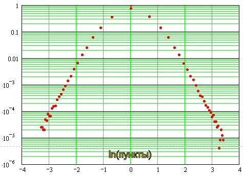
. On the bottom left is the probability distribution density, on the right - the same in logarithmic scale.
If the distribution were normal, we'd have a parabola here, which it isn't, because of the "fat" tails. In principle, we should fit a least-squares Gaussian here, then everything will fall into place. I'll have to throw in a formula for the optimum fit...
Sergei, what about the double logarithmic? I've been thinking about it for a while now...
I still can't test it out of modesty :)
Sergei, what about the double logarithmic? I've been thinking about it for some time now...
I'm too modest to check it out :)
It turns out so:
It can be seen that near zero, the distribution is close to normal, and then it goes to asymptotic in the form of straight lines, which in the double logarithmic scale indicates the exponential nature of the distribution of "tails". In other words about their "heaviness".