Hearst index - page 9
You are missing trading opportunities:
- Free trading apps
- Over 8,000 signals for copying
- Economic news for exploring financial markets
Registration
Log in
You agree to website policy and terms of use
If you do not have an account, please register
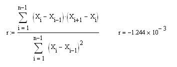
No, that's not it. According to this formula, it appears that the GVH is correlated. All the time r is around minus 0.5.
Here's the test code.
Checked it out.
Sergei, let's take it one step at a time.
1. We work with a BP similar to a quotation. Such a series is obtained by integrating CB with zero MO. Example of CB with zero MO:
dX=rnorm(n+1,0,10), where n+1 is number of CB members having Gaussian distribution, 0 is MO equal to zero in my case and 10 in your example, 10 is width of this distribution in my case and 100 in yours. To construct BP similar to the price one, we need to integrate the initial series (find its commutative sum):
Here is what the distribution of the increments of the integrated CB looks like (Fig. on the left) and the increments themselves on the background of BP (red and blue lines on the right Fig.):
Sergey, we are studying properties of BP (the blue one), while in your post, you have substituted the very first difference (dX in my notation and X in yours) into the formula to calculate the correlation coefficient of the first difference in the series. Of course, you will get R=0.5 and there should not be another one (it is proved elementary). So, if now to calculate by my proposed formula r for integrated CB with zero MO (the blue one in the right fig.), you will get the expected zero:
And, of course, this is the same as r for a series of dX increments (but, by a different formula):
I hope we now have a consensus on this point?
P.S. You could do it this way:
All right, let's get this straight.
I did what you said, I reintegrated the CB with MOJ=0. Here's all the code.
Seems to be ok at first glance. But there is a pitfall. Let's feed a correlated array to the input of the formula. As trend + noise. y=a*x+b+rnorm(). This may be simply done by setting 0.5 instead of MOJ=0.
From the figure you can see that the curve (blue) is clearly correlated. Having divided it into two arrays A and B, let us calculate the correlation coefficient, it turns out to be 0.993. According to your formula it is 0.225.
The matter is that by definition the correlation coefficient (CC) is counted between the two arrays. You're using the same one. You can do this by comparing an array to itself. It's called ACF, i.e. two arrays A are formed - initial, and the second B shifted in time relative to A, and a graph is built - the dependence of correlation coefficient on the shift. If there is no shift, the ACF of course = 1. Here is the ACF plot of the last blue curve.
This is the approximation. So, I still stick to my opinion that you are calculating by this formula, but it is not AC. The numbers don't add up.
But we have gone sideways. We must first calculate the Hurst correctly and then see how it differs from the QC.
Here is an interesting paper which analyses different time series
using the Hearst index.
The figure shows that the curve (blue) is clearly correlated. Splitting it into two arrays A and B, we find the correlation coefficient, which is 0.993. Your formula gives us 0.225.
Here I don't understand it completely.
Into what arrays did you divide the trend BP? Into a straight Y=a*X+b and a random component with zero MO, and between them you look for the correlation coefficient?
Here's an interesting paper that does an analysis of various time series
using Hearst's index.
I didn't get it all right here.
I get it now.
You are looking for the correlation coefficient between the original BP (not its increments) and the same BP, but shifted by 500 counts to the right. That is, you are looking for the correlation coefficient between two always positive BPs! Well, of course it will be positive and very large (about 1) always.
Sergey, I don't understand you! What do you count, the correlation coefficient between the initial BP and the same but shifted? What the hell do we need it for! We are interested in the correlation coefficient between neighboring samples in the series of the first difference of the initial BP. It is this coefficient that shows the dependence of the expected increment on the previous increments. It is this coefficient that is identical to Hurst shifted by 1/2.
>> Thank you. >> We'll see.
There seems to be some truthhere.
I tried to implement it, but I got very close to 1 for rates.
______________
Reread the article -- I think I'm on the wrong side of the coin.
For currency pairs Hearst's index should be calculated for the derivative, I calculated it for the exchange rate.
Reread the article -- sort of stepped on a rake.
Yeah:-)
Getting ahead of myself.
Here is how the series of the integrated SV and EURGBP rate looks (Fig. on the left), and here is how the amplitudes of their increments on different TFs in double logarithmic scale (Fig. on the right), on the abscissa axis the logarithm of the TF is plotted:
Hers, asserts that the tangent of the slope angle of these lines is equal to 1/2 for a random integrated variable (it makes no sense to trade on such a quotient), less than 1/2 for a pullback market and greater than 1/2 for a trend market. Let's see what this angle equals for NE. Here we can, as advised in the article, draw an ISC line and find its slope, but I will find this value locally - by drawing a line through every two points. The result will be a PC for each TF:
The circles here show the PC for the CB (red) and blue for the EURGBP quotient on the abscissa axis for the TF in min. The crosses show the correlation coefficient between neighbouring readings for the first difference of the original series with an offset of 1/2. The correlation coefficient was calculated according to the formula given in the first message of this page. It can be seen that the agreement between these two ways of estimating the predictability of BP is satisfactory, while the formulas in my case are much smaller (only one). Which is, in fact, what was required to be shown.
In addition, the Random series gave PX=1/2 and r=0 (there is a bias in the figure) as follows from the definition. For the quotient, a rolling trend (antipersistence) is clearly visible, the larger the smaller the TF.
Here we show PCB for CB (red) and in blue for EURGBP kotier on the abscissa axis the TF is plotted in min.
The random series gave PX=1/2 and r=0 (there is a bias in the figure) as follows from the definition. For the cotier we can clearly see a rolling trend (antipersistence), the larger the smaller the TF.
That's probably why the pips are so fond of the euro pound
I guess that's why the pipsmen are so fond of the euro pound.
It's obvious!
It's obvious!
Out of sheer curiosity - I'd like to find extremely persistent pairs,
or at least the conditions under which persistence occurs):