Loss functions

When starting training, it is necessary to choose methods for determining the quality of network training. Training a neural network is an iterative process. At each iteration, we need to determine how accurate the neural network calculations are. In the case of supervised learning, it refers to how much they differ from the reference. By knowing the deviation only can we understand how much and which way we need to adjust the synaptic coefficients.

Therefore, we need a certain metric that will impartially and mathematically accurately indicate the error of the neural network's performance.

At first glance, it is quite a trivial task to compare two numbers (the calculated value of the neural network and the target). But as a rule, at the output of a neural network, we get not one value, but an entire vector. To solve this problem, lets turn to mathematical statistics. Let us introduce a loss function that depends on the calculated value (y') and the reference value (y).

This function should determine the deviation of the calculated value from the reference value (error). If we consider the computed and target values as points in space, then the error can be seen as the distance between these points. Therefore, the loss function should be continuous and non-negative for all permitted values.

In an ideal state the calculated and reference values are the same, and the distance between the points is zero. Therefore, the function must be convex downwards with a minimum at L(y,y')=0.

The book "Robust and Non-Robust Models in Statistics " by L.B.Klebanov describes four properties that a loss function should have:

Completeness of information
The absence of a randomization condition
Symmetry condition
Rao-Blackwell state (statistical estimates of parameters can be improved)

The book presents quite a few mathematical theorems and their proofs. It demonstrates the relationship between the choice of loss function and a statistical estimate. As a consequence, certain statistical issues can be resolved through the proper choice of the loss function.

Mean Absolute Error (MAE) #

One of the earliest loss functions, the Mean Absolute Error (MAE), was introduced by the 18th-century French mathematician Pierre-Simon Laplace. He proposed using the absolute difference between the reference and computed values as a measure of deviation.

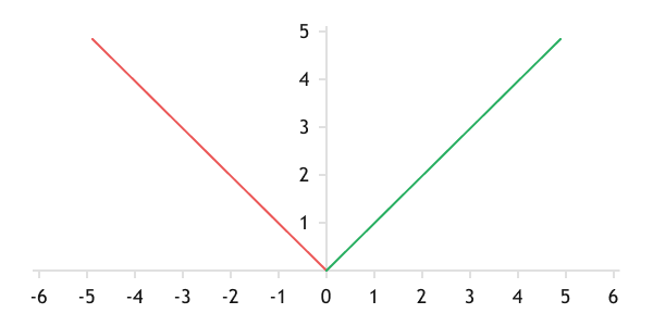
The function has a graph that is symmetric about zero, and linear before and after zero.

Graph of the Mean Absolute Deviation function

The use of Mean Absolute Error provides a linear approximation of the analytical function to the training dataset across the entire range of error.

Let's look at the implementation of this function in MQL5 program code. To calculate deviations, the function must receive two data vectors: calculated and reference values. This data will be passed as parameters to the function.

At the beginning of the method, we compare the size of the resulting arrays. Ideally, array sizes should be at least zero. If the check fails, we exit the function with a result of the maximum possible error, DBL_MAX.

double MAE(double &calculated[], double &target[])
  {
   double result = DBL_MAX;
//---
   if(calculated.Sizel() < target.Sizel() || target.Sizel() <= 0)
      return result;

After successfully passing the checks, we create a loop to accumulate the absolute values of deviations. In conclusion, we divide the accumulated sum by the number of reference values.

//---
   result = 0;
   int total = target.Size();
   for(int i = 0; i < total; i++)
      result += MathAbs(calculated[i] - target[i]);
   result /= total;
//---
   return result;
  }

Mean Squared Error (MSE) #

The 19th-century German mathematician Carl Friedrich Gauss proposed using the square of the deviation instead of the absolute value in the formula for mean absolute deviation. The function is called the standard deviation.

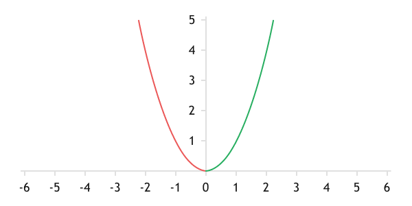
Thanks to squaring the deviation, the error function takes the form of a parabola.

Graph of the mean squared deviation function

When using mean squared deviation, the speed of error compensation is higher when the error itself is larger. When the error decreases, the speed of its compensation also decreases. In the case of neural networks, this allows for faster convergence of the neural network with large errors and finer tuning with small errors.

But there is a flip side to the coin: the property mentioned above makes the function sensitive to noisy phenomena, as rare, large deviations can lead to a bias in the function.

Currently, the use of mean squared error as a loss function is widely employed in solving regression problems.

The algorithm for implementing MSE in MQL5 is similar to implementing MAE. The only difference is in the body of the loop, where the sum of the squares of the deviations is calculated instead of their absolute values.

double MSE(double &calculated[], double &target[])
  {
   double result = DBL_MAX;
//---
   if(calculated.Size() < target.Size() || target.Size() <= 0)
      return result;

//---
   result = 0;
   int total = target.Size();
   for(int i = 0; i < total; i++)
      result += MathPow(calculated[i] - target[i], 2);
   result /= total;
//---
   return result;
  }

Cross-entropy #

For solving classification tasks, the cross-entropy function is most commonly used as the loss function.

Entropy is a measure of uncertainty in distribution.

Applying entropy shifts calculations from the realm of absolute values into the realm of probabilities. Cross-entropy defines the similarity of probabilities of events occurring in two distributions and is calculated using the formula:

where:

p(yi) = the probability of the ith event occurring in the reference distribution
p(yi') = the probability of the ith event occurring in the calculated distribution

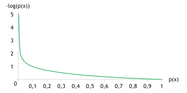
Since we are examining probabilities of events occurring, the probability values of an event always lie within the range of 0 to 1. The value of the logarithm in this range is negative, so adding a minus sign before the function shifts its value into the positive range and makes the function strictly decreasing. For clarity, the logarithmic function graph is shown below.

During training, for events in the reference distribution, when an event occurs, its probability is equal to one. The probability of a missing event occurring is zero. Based on the graph of the function, the event that occurred in the reference distribution but was not predicted by the analytical function will generate the highest error. Thus, we will stimulate the neural network to predict expected events.

It is the application of the probabilistic model that makes this function most attractive for classification purposes.

Graph of the logarithmic function

An implementation of this feature is presented below. The implementation algorithm is similar to the previous two functions.

double LogLoss(double &calculated[], double &target[])
  {
   double result = DBL_MAX;
//---
   if(calculated.Size() < target.Size() || target.Size() <= 0)
      return result;
//---
   result = 0;
   int total = target.Size();
   for(int i = 0; i < total; i++)
      result -= target[i] * MathLog(calculated[i]);
//---
   return result;
  }

Only three of the most commonly used loss functions are described above. But in fact, their number is much higher. And here, as in the case of activation functions, we will be assisted by vector and matrix operations implemented in MQL5, among which the Loss function is implemented. This function allows to compute the loss function between two vectors/matrices of the same size in just one line of code. The function is called for a vector or matrix of calculated values. The parameters of the function include a vector/matrix of reference values and the type of loss function.

double vector::Loss(
  const vector&       vect_true,    // true value vector
  ENUM_LOSS_FUNCTION  loss          // loss function type
   );

double matrix::Loss(
  const matrix&       matrix_true,  // true value matrix
  ENUM_LOSS_FUNCTION  loss          // loss function type
   );

MetaQuotes provides 14 readily implemented loss functions. These are listed in the table below.

Identifier	Description
LOSS_MSE	Mean squared error
LOSS_MAE	Average absolute error
LOSS_CCE	Categorical cross-entropy
LOSS_BCE	Binary cross-entropy
LOSS_MAPE	Average absolute error in percentages
LOSS_MSLE	Mean-squared logarithmic error
LOSS_KLD	Kulback-Leibler divergence
LOSS_COSINE	Cosine similarity/proximity
LOSS_POISSON	Poisson loss function
LOSS_HINGE	Hinge loss function
LOSS_SQ_HINGE	Quadratic piecewise linear loss function
LOSS_CAT_HINGE	Categorical piecewise linear loss function
LOSS_LOG_COSH	The logarithm of the hyperbolic cosine
LOSS_HUBER	Huber loss function

Neural network training

Error gradient backpropagation method