Neuron and principles of building neural networks

In their paper entitled "A logical calculus of the ideas immanent in nervous activity", Warren McCulloch and Walter Pitts proposed a mathematical model of a neuron and described the basic principles of neural network organization. The mathematical model of an artificial neuron involves two computation stages. Similar to a human neuron, in the mathematical model of an artificial neuron, the dendrites are represented by a vector of numerical values X, which is input into the artificial neuron. The dependence of the neuron value on each specific input is determined by the vector of weights, denoted as W. The first computation stage of the artificial neuron model is implemented as the product of the vector of initial signals by the vector of weights, which gives a weighted sum of initial data from the mathematical point of view.

where:

• n = number of elements in the input sequence
• wi = weight of the ith element of the sequence
• xi = the ith element of the input sequence

The weights determine the sensitivity of the neuron to changes in a particular input value and can be either positive or negative. This way, the operation of excitatory and inhibitory signals is simulated. The values of weights satisfying the solution of a particular problem are selected in the process of training the neural network.

As mentioned before, a signal appears on the axon of a neuron only after a critical value has accumulated in the cell body. In the mathematical model of an artificial neuron, this step is implemented by introducing an activation function.

Variations are possible here. The first models used a simple function to compare the weighted sum of input values with a certain threshold value. Such an approach simulated the nature of a biological neuron, which can be excited or at rest. The graph of such a neuron activation function will have a sharp drop in value at the threshold point.

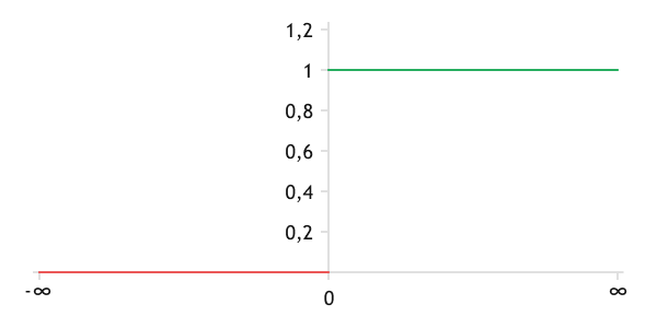
Graph of the threshold function of neuron activation.

In 1960, Bernard Widrow and Marcian Hoff published their work "Adaptive switching circuits", in which they presented the Adaline adaptive linear classification machine. This work has shown that using continuous neuron activation functions allows solving a wider range of problems with less error. Since then and up to our time, various sigmoid functions have been widely used as neuron activation functions. In this version, a smoother graph of the mathematical model of the neuron is obtained.

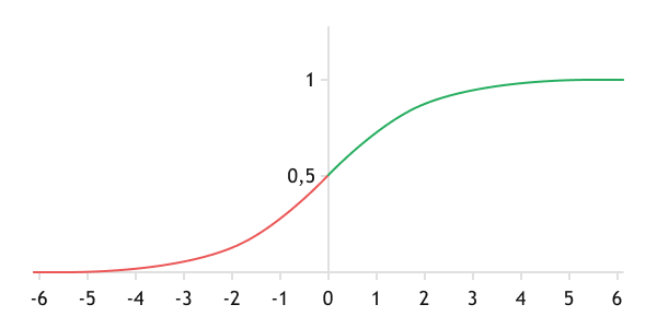
Graph of the logistic function (Sigmoid)

We will discuss different versions of activation functions and their advantages and disadvantages in the next chapter of the book. In a general form, the mathematical model of an artificial neuron can be schematically represented as follows.

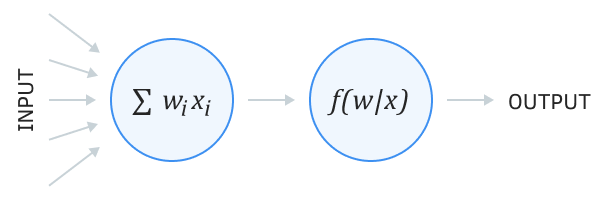
Scheme of the mathematical model of a neuron

This mathematical model of a neuron allows generating a logical True or False answer based on the analysis of input data. Let's consider the model's operation using the example of searching for the candlestick pattern "Pin Bar".

According to the classic Pin Bar model, the size of the candlestick "Nose" should be at least 2.5 times the size of the body and the second tail. Mathematically, it can be visualized as follows:

or

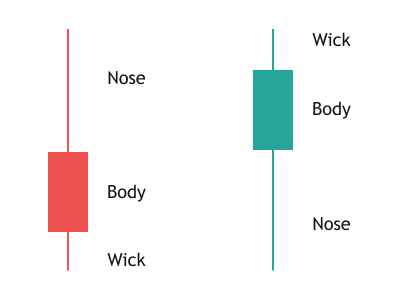
Pin Bar

According to the mathematical model of the neuron, we will input three values into the neuron: the size of the candlestick nose, body, and tail. The weights will be 1, -2.5, and -2.5, respectively. It should be noted that we will not consider weights when constructing the neural network. They will be selected during the training process.

The activation function will be a logical comparison of the weighted sum with zero. If the weighted sum of input values is greater than zero, the candlestick pattern is found and the neuron is activated. The output of the neuron is 1. If the weighted sum is less than zero, then the pattern is not found. The neuron remains deactivated and the output of the neuron is 0.

Now we have a neuron that will respond to the Pin Bar candlestick pattern. However, note that in a bullish pattern, the nose will be the lower tail, and in a bearish one, it will be the upper tail. That is, if we input a vector of values containing the upper tail, body, and lower tail of a candlestick, we need two neurons to define the pattern: one will define a bullish pattern and the other a bearish pattern.

Does this mean we will need to create a program for each pattern separately? No. We will combine them into a single neural network model.

In a neural network, all neurons are grouped into sequential layers. According to their location and purpose, neural layers are categorized into input, hidden, and output layers. There is always one input and one output layer, but the number of hidden layers can vary, depending on the complexity of the task at hand.

The number of neurons in the input layer corresponds to the number of inputs, which is three in our example: upper tail, body, and lower tail.

The hidden layer in our case consists of two neurons that define a bullish and a bearish pattern. The number of hidden layers and neurons in them is set during the design of the neural network and is determined by its architect depending on the complexity of the problem to be solved.

The number of hidden layers determines how the input data space is divided into subclasses. A neural network with a single hidden layer divides the input data space by a hyperplane. The presence of two hidden layers allows the formation of a convex region in the input data space. The third hidden layer allows the formation of almost any region in space.

The number of neurons in the hidden layer is determined by the number of sought-after features at each level.

The number of neurons in the output layer is determined by the neural network architect depending on the possible solution variants for the given task. For binary and regression problems, a single neuron may be sufficient. For classification tasks, the number of neurons will correspond to a finite number of classes.

An exception is a binary classification, where all objects are divided into two classes. In this case, one neuron is sufficient, since the probability of assigning an object to the second class P2 is equal to the difference between one and the probability of assigning an object to the first class P1.

In our example, the output layer will contain only one neuron, which will give the result: whether to open a trade or not, and in which direction. For this, we will assign a weight of 1 to the bullish pattern, and a weight of -1 to the bearish pattern. As a result, the buy signal will be 1, while the sell signal will be -1. Zero will mean there is no trading signal.

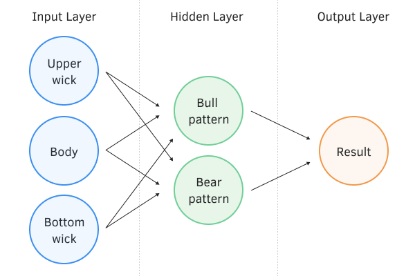
Perceptron model

Such a neural network model was proposed by Frank Rosenblatt in 1957 and was named Perceptron. This model is one of the first artificial neural network models. It is capable of establishing associative connections between input data and the resulting action. In real life, it can be compared to a person's reaction to a traffic light signal.

Of course, the perceptron is not without flaws; there are a number of limitations in its use. However, over the years of research, good results have been achieved in using the perceptron for classification and approximation tasks. Moreover, mechanisms for training the perceptron have been developed, which we will discuss shortly.