Machine learning methods

Among the built-in methods of matrices and vectors, there are several that are in demand in machine learning tasks, in particular, in the implementation of neural networks.

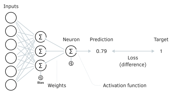
As the name implies, a neural network is a collection of many neurons which are primitive computing cells. They are primitive in the sense that they perform fairly simple calculations: as a rule, a neuron has a set of weight coefficients that are applied to certain input signals, after which the weighted sum of the signals is fed into the function, which is a nonlinear converter.

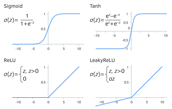
The use of an activation function amplifies weak signals and limits those that are too strong, preventing the transition to saturation (overflow of real calculations). However, the most important thing is that nonlinearity gives the network new computing capabilities, enabling the solution of more complicated problems.

Elementary neural network

The power of neural networks is manifested by combining a large number of neurons and establishing connections between them. Usually, neurons are organized into layers (which can be compared with matrices or vectors), including those with recursive (recurrent) connections, and can also have activation functions that differ in their effect. This makes it possible to analyze volumetric data using various algorithms, in particular, by finding hidden patterns in them.

Note that if it were not for the non-linearity in each neuron, a multilayer neural network could be represented in equivalent form as a single layer, whose coefficients are obtained by the matrix product of all layers (Wtotal = W1 * W2 * ... * WL, where 1..L are the numbers of layers). And this would be a simple linear adder. Thus, the importance of activation functions is mathematically substantiated.

Some of the most famous activation functions

One of the main classifications of neural networks divides them according to the learning algorithm used into supervised and unsupervised learning networks. Supervised ones require a human expert to provide the desired outputs for the original data set (for example, discrete markers of the state of a trading system, or numerical indicators of implied price increments). Unsupervised networks identify clusters in the data on their own.

In any case, the task of training a neural network is to find parameters that minimize the error on the training and test samples, for which the loss function is used: it provides a qualitative or quantitative estimate of the error between the target and the received network response.

The most important aspects for the successful application of neural networks include the selection of informative and mutually independent predictors (analyzed characteristics), data transformation (normalization and cleaning) according to the specifics of the learning algorithm, as well as network architecture and size optimization. Please note that the use of machine learning algorithms does not guarantee success.

Here, we will not go into the theory of neural networks, their classification, and typical tasks to be solved. This topic is too broad. Those interested can find articles on the mql5.com website and in other sources.

MQL5 provides three machine learning methods which have become part of the matrix and vector API.

• Activation calculates the values of the activation function
• Derivative calculates the values of the derivative of the activation function
• Loss  calculates the value of the loss function

Derivatives of activation functions enable the efficient update of model parameters based on the model error which changes during the learning process.

The first two methods write the result to the passed vector/matrix and return a success indicator (true or false), and the loss function returns a number. Let's present their prototypes (under the type object<T> we marked both, matrix<T> and vector<T>):

bool object<T>::Activation(object<T> &out, ENUM_ACTIVATION_FUNCTION activation)

bool object<T>::Derivative(object<T> &out, ENUM_ACTIVATION_FUNCTION loss)

T object<T>::Loss(const object<T> &target, ENUM_LOSS_FUNCTION loss)

Some activation functions allow setting a parameter with a third, optional argument.

Please refer to the MQL5 Documentation for the list of supported activation functions in the ENUM_ACTIVATION_FUNCTION enumeration and loss functions in the ENUM_LOSS_FUNCTION enumeration.

As an introductory example, let's consider the problem of analyzing the real tick stream. Some traders consider ticks to be garbage noise, while others practice tick-based high-frequency trading. There is an assumption that high-frequency algorithms, as a rule, give an advantage to big players and are based solely on the software processing of price information. Based on this, we will put forward a hypothesis that there is a short-term memory effect in the tick stream, due to the market makers' currently active robots. Then, a machine learning method can be used to find this dependence and to predict several future ticks.

Machine learning always involves putting forward hypotheses, synthesizing a model for them, and testing them in practice. Obviously, productive hypotheses are not always obtained. It is a long process of trial and error, in which failure is a source of improvement and new ideas.

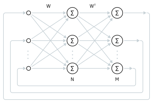
We will use one of the simplest types of neural networks: Bidirectional Associative Memory (BAM). Such a network has only two layers: input and output. A certain response (association) is formed in the output in response to the input signal. Layer sizes may vary. When the sizes are the same, the result is a Hopfield network.

Fully connected Bidirectional Associative Memory

Using such a network, we will compare N recent previous ticks and M next predicted ticks, forming a training sample from the near past to a given depth. Ticks will be fed into the network as positive or negative price increments converted to binary values [+1, -1] (binary signals are the canonical form of coding in BAM and Hopfield networks).

The most important advantage of BAM is the almost instantaneous (compared to most other iterative methods) learning process, which consists in calculating the weight matrix. We will give the formula below.

However, this simplicity also has a downside: the BAM capacity (the number of images that it can remember) is limited to the smallest layer size, provided that the condition of a special distribution of +1 and -1 in the training sample vectors is met.

Thus, for our case, the network will generalize all sequences of ticks in the training sample and then, in the course of regular work, it will roll down to one or another stored image, depending on the sequence of new ticks presented. How well this will turn out in practice depends on a very large number of factors, including the network size and settings, the characteristics of the current tick stream, and others.

Because it is assumed that the tick stream has only short-term memory, it is desirable to retrain the network in real time or close to it, since training is actually reduced to several matrix operations.

So, in order for the network to remember the associative images (in our case, the past and the future of the tick stream), the following equation is required:

where W is the weight matrix of the network. The summation is performed over all pairwise products of the input vectors Ai and corresponding output vectors Bi.

Then, when the network is running, we feed the input image to the first layer, apply the W matrix to it, and thereby activate the second layer, in which the activation function for each neuron is calculated. After that, using the transposed W T matrix, the signal propagates back to the first layer, where activation functions are also applied in neurons. At this moment, the input image no longer arrives at the first layer, i.e., the free oscillatory process continues in the network. It continues until the changes in the signal of the network neurons stabilize (i.e., become less than a certain predetermined value).

In this state, the second layer of the network contains the found associated output image — the prediction.

Let's implement this machine learning scenario in the script MatrixMachineLearning.mq5.

In the input parameters, you can set the total number of last ticks (TicksToLoad) requested from the history, and how many of them are allocated for testing (TicksToTest). Accordingly, the model (weights) will be based on (TicksToLoad - TicksToTest) ticks.

Also, in the input variables, the sizes of the input vector (the number of known ticks PredictorSize) and output vector (the number of future ticks ForecastSize) are selected.

Ticks are requested at the beginning of the OnStart function. In this case, we only work with Ask prices. However, you can also add Bid and Last process, along with volumes.

Let's split ticks into training and test sets.

To calculate price increments, we use the Convolve method with an additional vector {+1, -1}. Note that the vector with increments will be 1 element shorter than the original.

Convolution according to the VECTOR_CONVOLVE_VALID algorithm means that only full overlaps of vectors are taken into account (i.e., the smaller vector is sequentially shifted along the larger one without moving beyond its boundaries). Other types of convolutions allow vectors to overlap with only one element, or half of the elements (in this case, the remaining elements are beyond the corresponding vector and the convolution values show border effects).

To convert continuous values of increments into unit pulses (positive and negative depending on the sign of the initial element of the vector), we will use an auxiliary function Binary (not shown here): it returns a new copy of the vector in which each element is either +1 or -1.

Based on the received input sequence, we use the TrainWeights function to calculate the W neural network weight matrix. We will consider the structure of this function later. For now, please pay attention that the PredictorSize and ForecastSize parameters are passed to it, which enables the splitting of a continuous sequence of ticks into sets of paired input and output vectors according to the size of the input and output BAM layers, respectively.

Immediately after training the network, we check its accuracy on the training set: just to make sure that the network has been trained. This is implemented by the CheckWeights function.

However, it is more important to check how the network behaves on unfamiliar test data. To do this, let's differentiate and binarize the second vector ask2 and then also send it to CheckWeights.

It's time to get acquainted with the TrainWeights function, in which we define A and B matrices to "slice" vectors from the passed input sequence, i.e. from the data vector.

Each successive A pattern is obtained from consecutive ticks in quantity equal to predictor, and the future pattern corresponding to is obtained from the following response elements. As long as the total amount of data allows, this window shifts to the right, one element at a time, forming more new pairs of images. Images are numbered by rows, and ticks in them are numbered by columns.

Next, we should allocate memory for the weight matrix W and fill it using matrix methods: we sequentially multiply rows from A and B using Outer, and then perform matrix summation.

The CheckWeights function performs similar actions for a neural network, the weight coefficients of which are passed in a ready-made form in the first W argument. The sizes of the training vectors are extracted from the W matrix itself.

Matrices A and B in this case are not formed to calculate W but act as "suppliers" of vectors for testing. We also need a transposed copy of W to calculate the return signals from the second network layer to the first.

The number of iterations during which transient processes are allowed in the network, up to convergence, is limited by the limit constant.

Variables positive, negative, and average are needed to calculate the statistics of successful and unsuccessful predictions in order to evaluate the quality of training.

Further, the network is activated in a loop over test pattern pairs and its final response is taken. Each next input vector is written into vector a, and output layer b is filled with zeros. After that, iterations are launched for signal transmission from a to b using the matrix W and applying the activation function AF_TANH, as well as for the feedback signal from b to a, and also the use of AF_TANH. The process continues until reaching limit loops (which is unlikely) or until the convergence condition is fulfilled, under which the a and b neuron state vectors practically do not change (here we use the Compare method and auxiliary copies of x and y vectors from the previous iteration).

After reaching a stable state, we transfer the states of neurons from continuous (real) to binary +1 and -1 using the Binarize function (it is similar to the previously mentioned Binary function, but changes the state of the vector in place).

Now, we only need to count the number of matches in the output layer with the target vector. For this, perform scalar multiplication of vectors. A positive result means that the number of correctly guessed ticks exceeds the number of incorrect ones. The total hit count is accumulated in 'average'.

After the cycle is completed for all test samples, we display statistics.

The script also includes the RunWeights function which represents a working run of the neural network (by its weight matrix W) for the online vector from the last predictor ticks. The function will return a vector with estimated future ticks.

At the end of OnStart, we pause execution for 1 second (in order to wait for new ticks with a certain degree of probability), request the last PredictorSize + 1 ticks (do not forget +1 for differentiation), and make predictions for them online.

Running the script with the default settings on EURUSD on Friday evening gave the following results.

The symbol and time are not mentioned since the market situation can significantly affect the applicability of the algorithm and the specific network configuration. When the market is open, every time you run the script you will get new results as more and more ticks come in. This is an expected behavior consistent with the short memory formation hypothesis.

As we can see, the training accuracy is acceptable, but it noticeably decreases on test data and may fall below 50%.

At this point, we smoothly move from programming to the field of scientific research. The machine learning toolkit built into MQL5 allows you to implement many other configurations of neural networks and analyzers, with different trading strategies and principles for preparing initial data.