Implementing a convolutional model in Python

We will implement the convolutional models in the Python language using the tools provided by the Keras library from TensorFlow. This library offers several options for convolutional layers. First of all, these are the basic versions of convolutional layers:

• Conv1D
• Conv2D
• Conv3D

From the names of the objects representing convolutional layers, it can be inferred that they are intended for processing input data of various dimensions.

The Conv1D class objects create the core of the convolution that collapses with the original data in one dimension to create an output tensor. It is important to understand and not to get confused. The initial data is convoluted in one dimension, but the initial data supplied to the neural layer input must be in the form of a three-dimensional tensor. The first dimension determines the size of the package of the data (batch size) being processed. The second is measuring convolution. The third dimension contains the initial data for convolution.

As a result of data processing, the layer also returns a 3D tensor. The first dimension remains the same; it is equal to the size of the data package being processed. The second dimension varies depending on the specified convolution parameters. The third dimension will be equal to the specified number of filters used.

It should be understood that each filter applies to all initial data. At one time, the initial data is processed in the size of the third dimension multiplied by the size of the convolution window. This is a slight difference from our implementation of the convolutional layer in MQL5. There, we defined the convolution window as the number of elements, while here, the convolution window determines the number of elements in the second dimension of the three-dimensional tensor of input data.

One filter returns one value for each convolution window. Since the entire third dimension is involved in the convolution process, we get one element from each filter. As a result, the size of the third dimension of the output tensor changes by the number of filters used.

Like a fully connected layer, the convolutional layer class offers a fairly wide range of parameters for fine-tuning the operation. Let's take a look at them.

• filters — the number of filters used in the bundle.
• kernel_size — one-dimensional convolution window size.
• strides — the size of the convolution step.
• padding — one of the following values is allowed: "valid", "same" or "causal" (case-insensitive); "valid" means no indentation; "same" causes the input data to be evenly filled with zeros to obtain an output size equal to the input size; "causal" leads to the emergence of causal (extended) changes, for example, output [t] does not depend from input [t+1:]. It's useful when modeling temporal data, where the model must not violate the temporal order.
• data_format — one of the following values is allowed: “channels_last” or “channels_first”; determines which dimension of the input tensor contains data for convolution; the default is “channels_last”.
• dilation_rate — used for advanced convolution and determines the expansion rate.
• groups — the number of groups into which the input is divided along the channel axis; each group is collapsed separately using filters, and the output is a combination of all results along the channel axis.
• activation — activation function.
• use_bias — indicates whether to use a bias vector.
• kernel_initializer — sets a method for initializing the weight matrix.
• bias_initializer — sets the method for initializing the displacement vector.
• kernel_regularizer — indicates a method for regularizing the weight matrix.
• bias_regularizer — indicates a method for regularizing the displacement vector.
• activity_regularizer — indicates a method for regularizing results.
• kernel_constraint — specifies the restriction function for the weight matrix.
• bias_constraint — specifies the constraint function for the displacement vector.

For timeseries, it is usually suggested to use a one-dimensional Conv1D convolution. Convolution is carried out by time intervals. At the same time, each filter checks for its own pattern in a specific time interval. In relation to solving our problem, filters will assess the status of all indicators used within the number of candles specified by the strides parameter. The process of convolution, like the neurons of a fully connected layer, does not assess the mutual influence of individual components of the initial data. It only assesses the similarity of the initial data with a given pattern. Of course, we don't explicitly define these patterns when constructing the neural network. We select them during the training process. However, it is assumed that during practical application, these patterns will remain static between retraining periods.

True, convolutional layers are more resistant to various distortions of the initial data due to the fact that small individual blocks are studied meticulously. However, it may be necessary to study the patterns of individual indicators. To solve this problem, we may need to use convolutional layers of a different dimension.

For example, Conv2D objects operate with convolutions with input data in two dimensions. At the same time, it should be understood that the difference between one-dimensional and two-dimensional convolutional layers goes beyond just their names. Objects in a two-dimensional convolutional layer expect a four-dimensional tensor at the input. By analogy with the Conv1D tensor, the first dimension determines the batch size, the second and third dimensions determine the convolution dimensions and the fourth dimension contains the initial data for convolution. Here arises a valid question: where do we obtain the data for another dimension? How do we divide our initial data set into four dimensions? We need to translate our raw data from a flat table to a voluminous table. The simplest solution is on the surface. We say that the depth of the table of the initial data is 1. Before declaring the two-dimensional neural layer, let's change the dimensionality of the tensor input to the Conv2D convolutional layer to a four-dimensional one by specifying a size of 1 for the fourth dimension.

Note that since the fourth dimension is 1, the length of the input data vector for convolution is 1. Therefore, for the convolution process to be effective, the convolution window needs to be greater than 1 in at least one dimension.

We will not dwell too much on the parameters of the Conv2D convolutional layer, since they are identical to the parameters of a one-dimensional array. The only differences are in the kernel_size, strides and dilation_rate parameters, which, in addition to a scalar value, can take a vector of two elements. Each element of such a vector contains parameter values for the corresponding dimension. At the same time, these parameters can take scalar values. In this case, the specified value will be used for both dimensions.

For more complex architectural solutions for neural networks, it may be necessary to use Conv3D 3D convolutional layers. Their usage can be justified, for example, in building arbitrage trading systems, where a separate dimension might be needed to segregate input data by instruments.

Just like in the case of a two-dimensional convolutional layer, using three-dimensional space requires increasing the dimensionality of the input data. A five-dimensional tensor is expected at the Conv3D input.

The parameters of the Conv3D class, however, are inherited from the aforementioned classes with minimal changes. The only difference is in the size of the vectors of the convolution window and its pitch.

Attention should be paid to another feature of the convolution process. When performing operations, it is possible to both reduce the size of the data tensor (data compression) and increase it. The first approach is useful when dealing with large datasets, where it's necessary to extract a specific component from the overall volume of input information. This is frequently employed in computer vision tasks, where in high-resolution images, each pixel represents an individual value within the overall tensor of input data.

The second approach, increasing the dimensionality, can be beneficial when there's an insufficient amount of input data. In such cases, a small volume of input data needs to be split into separate components while searching for non-obvious dependencies.

It should be noted that this is not a complete list of convolutional layers offered by the Keras library. But it is beyond the scope of this book to describe all the library's features. You can always check them out on the library website. There you can also find the latest version of the library and instructions for installing and using it.

Just like convolutional layers, the Keras library offers several class options for a pooling layer. Among them are:

• AvgPool1D — one-dimensional data averaging.
• AvgPool2D — two-dimensional data averaging.
• AvgPool3D — three-dimensional data averaging.
• MaxPool1D — one-dimensional extraction of the maximum value.
• MaxPool2D — two-dimensional extraction of the maximum value.
• MaxPool3D — three-dimensional extraction of the maximum value.

All of these pooling layers have the same set of parameters:

• pool_size — an integer number or vector of integers, determines the window size.
• strides — an integer number or vector of integers, determines the window pitch.
• padding — means one of the following values is allowed: "valid", "same" or "causal" (case-insensitive); "valid" means no indentation; "same" — causes the source data to be evenly filled with zeros to obtain an output size equal to the input size.
• data_format — one of the following values is allowed: "channels_last" or "channels_first"; determines which dimension of the input tensor contains data for convolution; the default is "channels_last".

We will also implement convolutional neural network models in our template. Just like when testing perceptron models, we will create three neural network models with different architectures and compare the results of their training. Therefore, for implementation, we will take the previously created file perceptron.py and create a copy of it called convolution.py. In this created file, we will replace the model declaration blocks.

First, we will create a perceptron with three hidden layers and weight matrix regularization. It will serve as a basis for comparing the performance of convolutional neural networks to the results of training a fully connected perceptron.

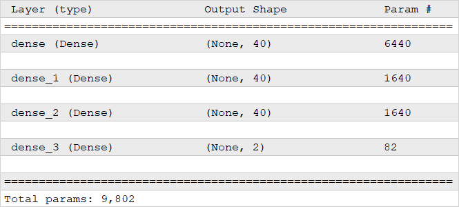
This model has 9802 parameters. The screenshot below shows the structure of the neural network we created. In the first column of the table, the name and type of the neural layer are indicated, while in the second column, the tensor dimensionality of the results for each layer is specified. Note that the first dimension is not set; None is specified instead of the size. This means that this dimension is not strictly defined and can be of variable length. This dimension is set by the batch size of the data patch. The third column shows the number of parameters in the weight matrix for each layer.

In the second model, we will insert a one-dimensional Conv1D convolution layer with 8 filters immediately after the initial data, and specify the convolution window and step as 1. Such a layer will roll up all specified indicators within a single candlestick. In doing so, let's not forget to change the dimensionality of the input data tensor from two-dimensional to three-dimensional.

Note that although we're transferring data to a 3D tensor, we specify two dimensions in the Reshape layer parameters. This is due to the fact that the first dimension of the tensor is variable and is set by the batch size of the input data batch.

And one more thing. The dimensional vector passed in the parameters of the Reshape class contains −1 in the first dimension. This tells the class to independently calculate the size of this dimension based on the size of the original data tensor and the specified dimensions of other dimensions.

Behind the convolutional layer, we will place a one-dimensional subsample layer with a choice of the maximum MaxPool1D value. As mentioned above, the convolutional layer operates with three-dimensional tensors. At the same time, the subsequent fully connected layers work with two-dimensional tensors. Therefore, for the proper functioning of fully connected layers, we need to return the data to a two-dimensional dimensionality. To do this, we will use the neural layer of the Flatten class.

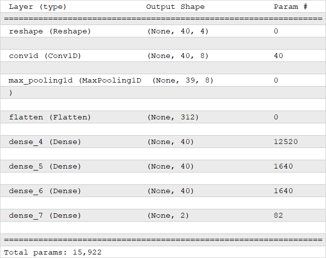
Note: In the initial data, each candlestick is described by four values. The use of eight filters increases the dimensionality of the processed tensor. As a result, the model with a one-dimensional convolutional layer already contains 15,922 parameters.

In the third model, we will replace a 1 one-dimensional convolution layer with a two-dimensional one. As a result, we will change the pooling layer and the data dimension. As mentioned above, we will set the fourth dimension to 1. We can now control the size of the convolution window in two dimensions: time and indicator. Since we would like to assess different patterns in the readings of each individual indicator, we will specify the size of the convolution window in the first temporal dimension as 3 (evaluating patterns from 3 consecutive candlesticks), and the size of the window in the second dimension of indicators as 1. This will allow us to identify patterns in the movement of each indicator separately. The pitch of the convolution window in both directions will be set to 1.

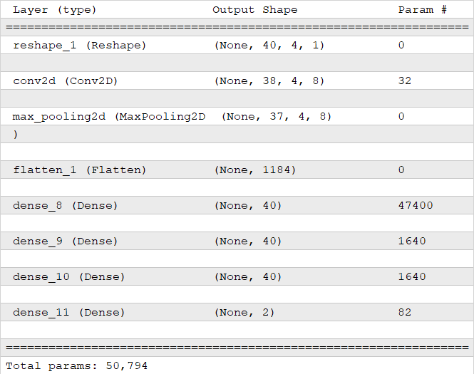
With these parameters, the first dimension (time dimension) will decrease by two elements as a result of the convolution operations. The second dimension (dimension of indicators) will remain unchanged since the convolution window and its pitch in this dimension are 1. At the same time, we will increase the third dimension, and it will become equal to the number of filters. Let me remind you that before the convolution operation, the third dimension was equal to 1. As a result of all iterations, the number of network parameters increased to 50,794. The structure of the new neural network is presented below. As you can see, the convolution layer has only 32 parameters. Such an increase in the number of network parameters is due to the enlargement of the tensor size after the convolution operation for the reasons mentioned above. This can be seen from the number of parameters in the first fully connected layer after convolution.

The rest of our script will remain unchanged. We will learn more about the script results in the next section.