- Principles of batch normalization implementation
- Building a batch normalization class in MQL5
- Organizing multi-threaded computations in the batch normalization class
- Implementing batch normalization in Python
- Comparative testing of models using batch normalization
Comparative testing of models using batch normalization
We have done a lot of work together and created a new class for batch normalization implementation. Its main purpose is to solve the internal covariance shift problem. As a result, the model should learn faster and the results should become more stable. Let's do some experiments and see if that's the case.
First, we will test the model using our class written in MQL5. For experiments, we will use very simple models that consist of only fully connected layers.
In the first experiment, we will try to use a batch normalization layer instead of pre-normalization in the data preparation stage. This approach will reduce the cost of data preparation both for model training and during commercial operation. In addition, the inclusion of normalization in the model allows it to be used with real-time data streams. This is how stock quotes are delivered, and processing them in real-time gives you an advantage.
To test the approach, we will create a script that uses one fully connected hidden layer and a fully connected layer as the neural layer of the results. Between the hidden layer and the initial data layer, we will set up a batch normalization layer.
The task is clear, so let's move on to practical implementation. To create the script, we will use the script from the first test of a fully connected perceptron perceptron test.mq5 as a base. Let's create a copy of the file with the name perceptron_test_norm.mq5.
At the beginning of the script are the external parameters. We will transfer them to the new script without any changes.
//+------------------------------------------------------------------+
|
In the script, we will only make changes to the CreateLayersDesc function that serves to specify the model architecture. In the parameters, this function receives a pointer to a dynamic array object, which we are to fill with descriptions of the neural layers to be created. To exclude possible misunderstandings, let's clear the obtained dynamic array immediately.
bool CreateLayersDesc(CArrayObj &layers)
|
First, we create a layer to receive the initial data. Before passing the description of the layer to be created, we must create an instance of the neural layer description object CLayerDescription. We create an instance of the object and immediately check the result of the operation. Please note that in case of an error, we display a message to the user, then we delete the dynamically created array object that was created earlier and only then terminate the program execution.
When the object is successfully created, we begin populating it with the desired content. For the initial data neural layer, we specify the basic type of a fully connected neural layer with zero initial data window without activation function and parameter optimization. We specify the number of neurons to be sufficient to receive the entire sequence of the pattern description. In this case, the number is equal to the product of the number of neurons in the pattern description by the number of elements in one candlestick description.
descr.type = defNeuronBase;
|
Once all the parameters of the created neural layer are specified, we add our neural layer description object to the dynamic array of the model architecture description and immediately check the result of the operation.
if(!layers.Add(descr))
|
After adding the description of a neural layer to the dynamic array, we proceed to the description of the next neural layer. Again, we create a new instance of the neural layer description object and check the result of the operation.
//--- batch normalization layer
|
The second layer of the model will be the batch normalization layer. We will tell the model about this by specifying an appropriate constant in the type field. We specify the number of neurons and the size of the initial data window according to the size of the previous neuron layer. A new batch size parameter is added for the batch normalization layer. For this parameter, we will specify a value equal to the batch size between updates of the batch parameters. We do not use the activation function, but we specify a method to optimize the Adam parameters.
descr.type = defNeuronBatchNorm;
|
After specifying all the necessary parameters of the new neural layer, we add it to the dynamic array of the model architecture description. As always, we check the result of the operation.
if(!layers.Add(descr))
|
Next in our model, there is a block of hidden layers. The number of hidden layers is specified in the external script parameters by the user. All hidden layers are basic fully connected layers with the same number of neurons, which is specified in the external parameters of the script. Therefore, to create all the hidden neural layers, you only need one description object for the neural layer, which can be added multiple times to the dynamic array describing the model architecture.
Hence, the next step is to create a new instance of the neural layer description object and check the result of the operation.
//--- block of hidden layers
|
After creating the object, we fill it with the necessary values. Also, we specify the base type of the neuron layer defNeuronBase. The number of elements in the neural layer is transferred from the external parameter of the HiddenLayer script. We will use Swish as the activation function and Adam as the parameter optimization method.
descr.type = defNeuronBase;
|
Once sufficient information is provided for creating a neural layer, we organize a loop with the number of iterations equal to the number of hidden layers. Within the loop, we will add the created description of the hidden neural layer to the dynamic array describing the model architecture. At the same time, don't forget to control the process of adding the description object to the array at each iteration.
for(int i = 0; i < HiddenLayers; i++)
|
In conclusion of the model description, you need to add the description of the output neural layer. For this, we create another instance of the neural layer description object and immediately check the result of the operation.
//--- layer of results
|
After creating the object, we fill it with the description of the neural layer to be created. For the output layer, you can use the basic type of fully connected neural layer with two elements (corresponding to the number of target values for the pattern). We use the linear activation function and the Adam optimization method as we did for the other model layers.
descr.type = defNeuronBase;
|
Add the prepared description of the neural layer to the dynamic array describing the architecture of the model.
if(!layers.Add(descr))
|
And of course, don't forget to check the result of the operation
This concludes our work on building the script to run the first test, while the rest of the script code is transferred to this one in an unchanged form. We will run the script on the previously prepared training dataset. I will remind you that for the purity of experiments, all models within this book are trained on a single training dataset. This applies to models created in the MQL5 environment and those written in Python.
From the test results presented in the figures below, it can be confidently stated that the use of batch normalization layers can effectively replace the preprocessing normalization procedure at the data preparation stage.
The direct impact of batch normalization layers can be assessed by comparing the error dynamics graph of a model without a batch normalization layer when trained on a non-normalized training dataset. The gap between the charts is enormous.
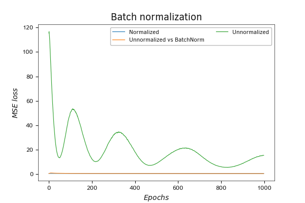
Batch normalization of initial data
At the same time, differences in the error dynamics graphs of the model during training on normalized data and on non-normalized data with the use of batch normalization layers may only become apparent when you zoom in on the graph. Only at the beginning of training, there is a gap between the performance of the models. As training iterations increase, the accuracy gap of the models shrinks dramatically. After 200 iterations, the model using the normalization layer shows even better performance. This further confirms the possibility of including batch normalization layers in a model for real-time data normalization, providing additional evidence of its effectiveness.
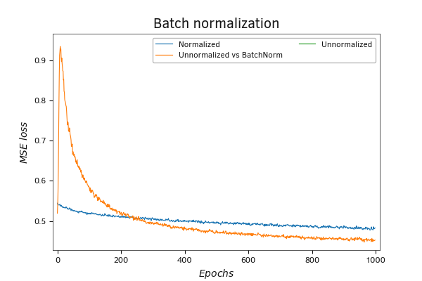
Batch normalization of initial data
We performed a similar experiment with models created in Python. This experiment confirmed the earlier findings.
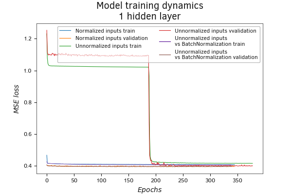
Batch normalization of initial data (MSE)
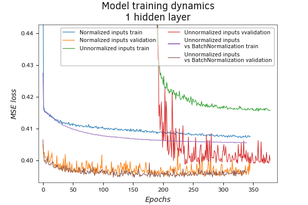
Batch normalization of initial data (MSE)
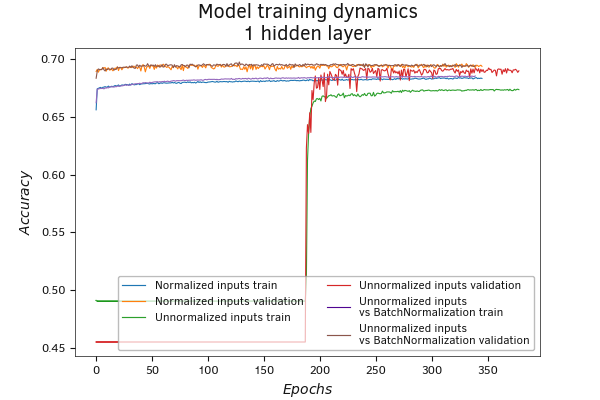
Batch normalization of initial data (Accuracy)
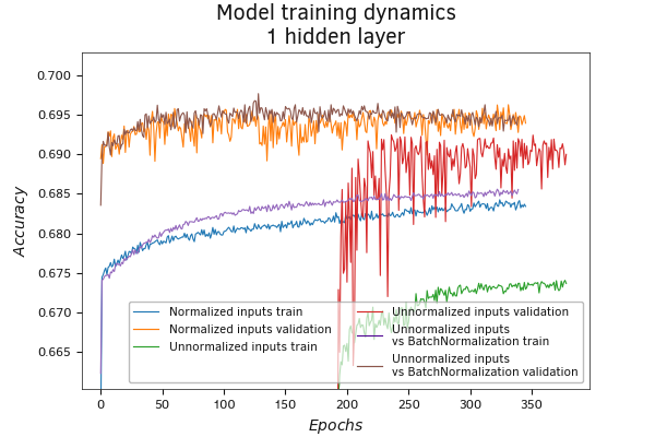
Batch normalization of initial data (Accuracy)
Furthermore, within the scope of this experiment, the model using batch normalization layers demonstrated slightly better results both on the training dataset and during validation.
The analysis of the graph for the Accuracy metric suggests similar conclusions.
The second and probably the main option for using a batch normalization layer is to put the batch normalization layer before the hidden layers. The authors proposed using this method in exactly this way to address the problem of internal covariate shift. To test the effectiveness of this approach, let's create a copy of our script with the name perceptron_test_norm2.mq5. We will make small changes in the block of creating hidden layers. This is because, in the new script, we need to alternate between fully connected hidden layers and batch normalization layers, so we will include the creation of batch normalization layers within the loop.
//--- Batch Normalization Layer
PrintFormat("Error adding layer: %d", GetLastError());
|
Otherwise, the script remains unchanged.
Testing of the script operation fully confirmed the earlier conclusions. Initially, when trained on non-normalized data, the model with batch normalization takes a little time to adapt. However, the gap in the accuracy of the models is shrinking dramatically.
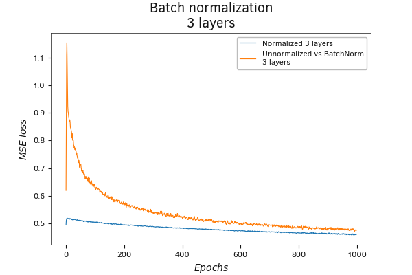
Batch normalization before the hidden layer
With a closer look, it becomes clear that the model with three hidden layers and batch normalization layers before each hidden layer even performs better on non-normalized input data. At the same time, its error dynamics graph decreases at a faster rate compared to the rest of the models.
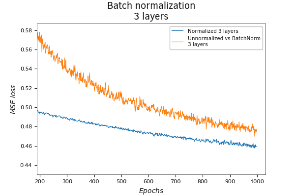
Batch normalization before the hidden layer
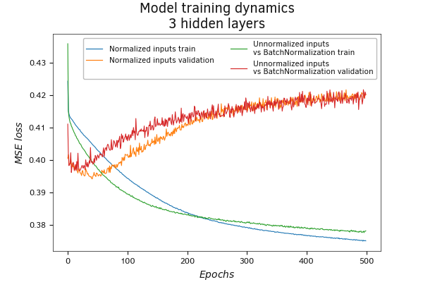
Batch normalization before the hidden layer (MSE)
Conducting a similar experiment with models created in Python also confirms that models using batch normalization layers before each hidden layer, under otherwise equal conditions, train faster and are less prone to overfitting.
The dynamics of changes in the Accuracy metric value also confirms the earlier conclusions.
Additionally, we validated the models on a test dataset to evaluate the performance using new data. The results obtained showed a fairly smooth performance of all four models. The divergence of the RMS error of the models did not exceed 5*10-3. Only a slight advantage was shown by models with three hidden layers.
Evaluation of the models using the Accuracy metric showed similar results.
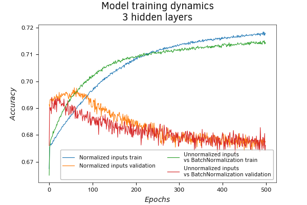
Batch normalization before the hidden layer (Accuracy)
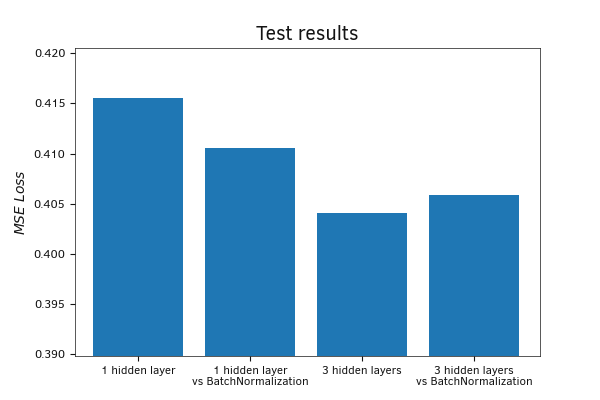
Testing the effectiveness of batch normalization on new data
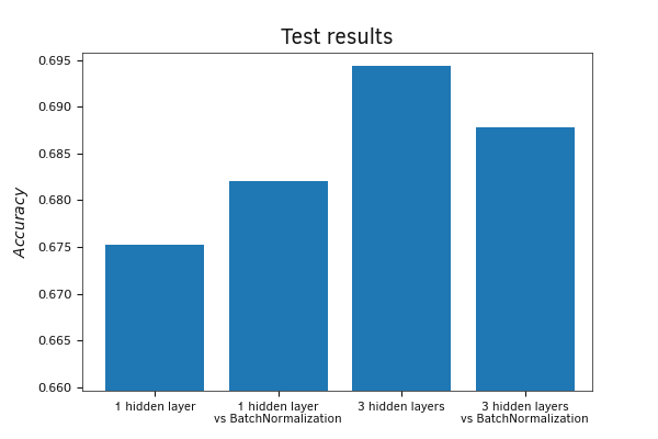
Testing the effectiveness of batch normalization on new data
To conclude, I decided to perform one more test. The authors of the method claim that the use of a batch normalization layer can increase the learning rate to speed up the process. Let's test this statement. We will run the perceptron_test_norm2.mq5 script again, but this time increase the learning rate by 10 times.
Testing has shown the potential effectiveness of this approach. In addition to a faster learning process, we got a better learning result than the previous ones.
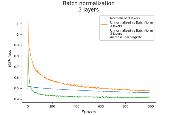
Batch normalization before the hidden layer with increased learning rate
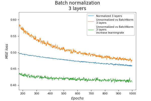
Batch normalization before the hidden layer with increased learning rate
In this section, we conducted a series of training tests for various models using batch normalization layers and without them. The obtained results demonstrated that a batch normalization layer after the input data can replace the normalization process at the data preparation stage for training. This approach allows the data normalization process to be built into the model and tuned during model training. In this way, we can process the initial data in real-time during the operation of the model without complicating the overall decision-making program.
In addition, using a batch normalization layer before the hidden model layers can speed up the learning process, all other things being equal.