Population optimization algorithms: Spiral Dynamics Optimization (SDO) algorithm

Contents

1. Introduction
2. Algorithm
3. Test results

1. Introduction

The scientific literature presents a wide variety of metaheuristic optimization algorithms based on various aspects of nature and populations. These algorithms are classified into several categories, for example: swarm intelligence, physics, chemistry, social human behavior, plants, animals and others. There are many metaheuristic optimization algorithms based on swarm intelligence. Algorithms based on physical phenomena are also widely proposed and successfully used in various fields.

Algorithms based on swarm intelligence incorporate elements of intelligence into the process of finding the optimal solution. They model the behavior of a swarm or colony, where individual agents exchange information and cooperate to achieve a common goal. These algorithms can be efficient in problems that require global search and adaptability to changing conditions.

On the other hand, physics-based algorithms rely on the laws and principles of physics to solve optimization problems. They simulate physical phenomena such as gravity, electromagnetism or thermodynamics and use these principles to find the optimal solution. One of the main advantages of physics-based algorithms is their ease of interpretation. They can accurately and consistently display dynamics across the entire search area.

In addition, some physics-based algorithms use the golden ratio, a mathematical and natural ratio that has special properties and helps converge quickly and efficiently to an optimal solution. The golden ratio has been studied and applied in various fields, including optimization of artificial neural networks, resource allocation and others.

Thus, physics-based metaheuristic optimization algorithms provide a powerful tool for solving complex optimization problems. Their precision and application of fundamental physical principles make them attractive to various fields where efficient search for optimal solutions is required.

Spiral Dynamics Optimization (SDO) is one of the simplest physics algorithms proposed by Tamura and Yasuda in 2011 and developed using the logarithmic spiral phenomenon in nature. The algorithm is simple and has few control parameters. Moreover, the algorithm has high computation speed, local search capability, diversification at an early stage and intensification at a later stage.

There are many spirals available in nature, such as galaxies, auroras, animal horns, tornadoes, seashells, snails, ammonites, chameleon tails or seahorses. Spirals can also be seen in ancient art created by humanity at the dawn of its existence. Over the years, several researchers have made efforts to understand spiral sequences and complexities, and to develop spiral equations and algorithms. A frequently occurring spiral phenomenon in nature is the logarithmic spiral observed in galaxies and tropical cyclones. Discrete logarithmic spiral generation processes were implemented as efficient search behavior in metaheuristics, which inspired the development of a spiral dynamics optimization algorithm.

Patterns called visible spiral sequences found in nature represent plants, trees, waves and many other shapes. Visual patterns in nature can be modeled using chaos theory, fractals, spirals and other mathematical concepts. In some natural patterns, spirals and fractals are closely related. For example, the Fibonacci spiral is a variant of the logarithmic spiral based on the golden ratio and Fibonacci numbers. Since it is logarithmic, the curve looks the same at every scale and can also be considered a fractal.

The above-mentioned patterns have inspired researchers to develop optimization algorithms. There are different types of spiral trajectories, here are the main ones:

• Archimedean spiral
• Cycloid spiral
• Epitrochoid helix
• Hypotrochoid spiral
• Logarithmic spiral
• Rose spiral
• Fermat's spiral

Each of these types of spirals has its own unique properties and can be used to model various natural patterns. Particular attention is paid to highlighting various nature-inspired optimization algorithms based on the concept of spiral paths. Over the years, researchers have developed various new optimization algorithms that make use of spiral motion.

Additionally, the behavior of non-spiral algorithms can be modified by using spiral paths as a superstructure or complement to improve the accuracy of the optimal solution.

The two-dimensional spiral optimization algorithm proposed by Tamura and Yasuda is a multi-point metaheuristic search method for two-dimensional continuous optimization problems. Tamura and Yasuda then proposed n-dimensional optimization using the philosophy of two-dimensional optimization.

2. Algorithm

The SDO algorithm for searching in multidimensional spaces, described by the authors, has limitations and disadvantages:

• Inapplicability for one-dimensional and other optimization problems with odd dimensions.
• Linking coordinates in pairs by the algorithm can affect the quality of the solution on specific problems and show false-positive results on synthetic tests.

Constructing spiral trajectories in multidimensional space presents certain difficulties. Thus, if the problem is limited to one-dimensional space, then a spiral cannot be constructed in the usual sense, since a spiral requires movement in at least two dimensions. In this case, we can use a simple function to change the coordinate value over time without using a spiral. If we are talking about a one-dimensional optimization problem, then the spiral is not used, since there are no additional dimensions for movement along the spiral.

In multidimensional space, spirals can be constructed for each pair of coordinates, but for the one remaining coordinate, a spiral cannot be defined. For example, in the case of a 13-dimensional space, it is possible to construct spirals for 6 pairs of coordinates, but one coordinate will move without a spiral component.

To construct spirals in multidimensional space, we can use the "multidimensional spiral" or "hyperspiral" method. This method involves introducing additional virtual coordinates and defining the spiral shape in each dimension. To construct a hyperspiral, we can use rotation matrices and algorithms based on the geometry of multidimensional spaces. However, this approach requires more complex calculations and may be difficult to implement in practical optimization problems.

Since the articles use multidimensional functions in the form of repeatedly duplicated two-dimensional ones, the original SDO can show unreasonably high results, because it uses pairwise coordinate binding. Thus, the spiral algorithm will show poor results on other multidimensional problems, where the coordinates are in no way related to each other. In other words, in this case, we will unintentionally create perfect conditions on duplicated functions for the spiral algorithm.

To avoid the above problems with the spiral algorithm, I propose an approach based on the projection of a two-dimensional spiral onto one coordinate axis. If we consider the motion of a point on a two-dimensional spiral as the motion of a pendulum, then the projection of the point motion onto each of the two coordinates will adhere to the projection of the pendulum motion onto each of the coordinates. Thus, we can use the projection of the pendulum point motion onto each of the axes in multidimensional space to simulate the point spiral motion in two-dimensional space.

When using the method of constructing spirals that simulate the behavior of a pendulum at each coordinate in a multidimensional space, the radius of each "virtual" spiral can be different. This can have a positive effect on the quality of the optimization, since some coordinates may be closer to known optima and do not need to be changed significantly.

We can take any law of harmonic vibrations with damping as a projection of a two-dimensional spiral onto a one-dimensional axis. I have selected a simple damped harmonic oscillator (the dependence of the point position on time) with the following equation:

x(t) = A*e^(-γt)*cos(ωt + φ)

where:

• A - amplitude of oscillations
• γ - damping ratio
• ω - oscillator natural frequency
• φ - initial phase of oscillations

The equation makes it clear that the damping ratio, frequency and initial phase are constants and can be used as algorithm inputs, but we will use not three, but two parameters. We will use the initial phase of the oscillations as a random component at each iteration (each coordinate will be slightly shifted in phase relative to other coordinates), otherwise the algorithm is completely deterministic and depends only on the initial placement of points in space.

The idea is that as soon as a new best global extremum is discovered, a new amplitude will be calculated for all points, which is the difference between the coordinate of the global extremum and the corresponding coordinate of the point. From this point on, the amplitudes along the coordinates are individual and stored in the memory of each point until a new better extremum is discovered and new amplitudes are determined.

After determining the amplitudes, each point begins to oscillate with attenuation, where the axis of symmetry of oscillations is the known coordinate of the global optimum. It is visually convenient to evaluate the influence of damping ratios and frequency (external parameters) using Figures 1 and 2.

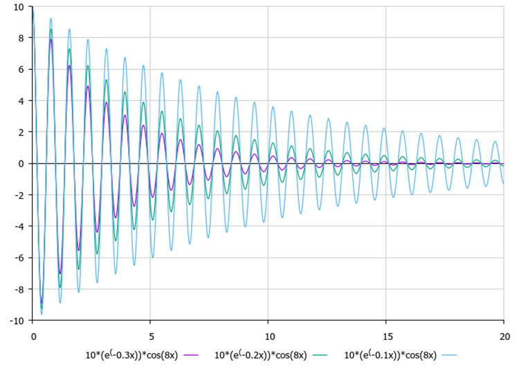
Figure 1. The influence of the amplitude on the nature of oscillations

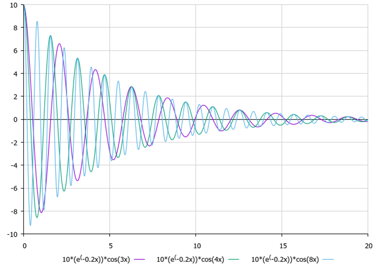
Figure 2. The influence of the frequency on the nature of oscillations

Although in our algorithm all coordinates are absolutely independent, as was mentioned, there are no pairwise combinations and connections between them in the logic for constructing spirals. If we constructed the movement of a point on a two-dimensional plane, we would obtain a spiral of the following type, as in Figure 3.

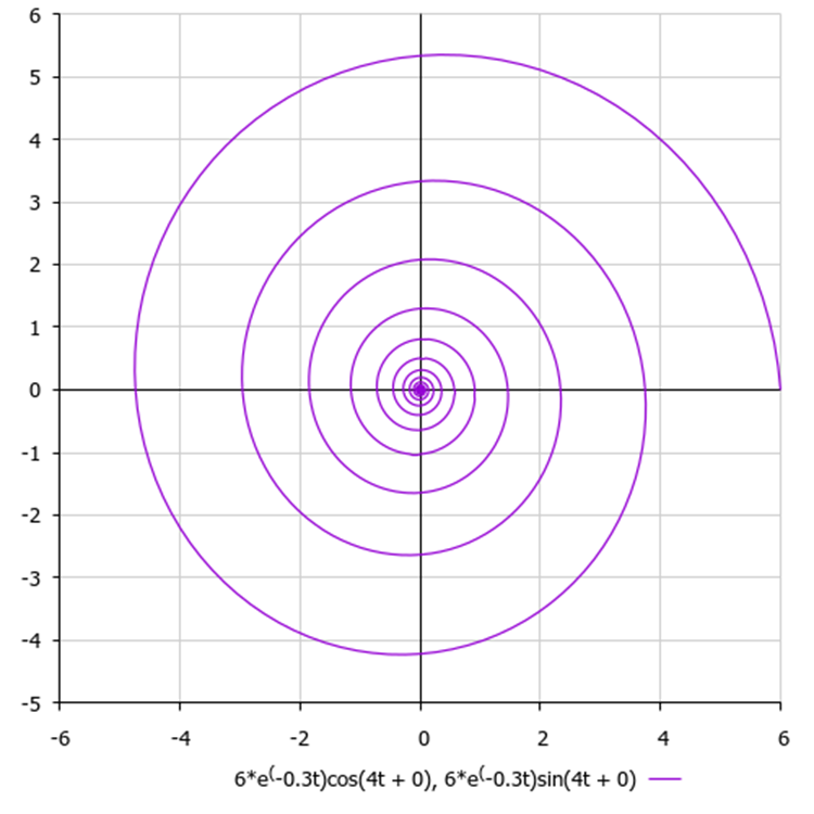
Figure 3. A hypothetical spiral with default algorithm parameters, where 6 is the amplitude value, 0.3 is the damping ratio and 4 is the frequency

In fact, in real problems, as well as in test functions, the amplitudes along each of the coordinates do not have to be the same (unlike the original algorithm). The difference in amplitudes will produce flattened spirals. With a smaller amplitude, the corresponding coordinate will be refined faster, since it is closer to the known best value.

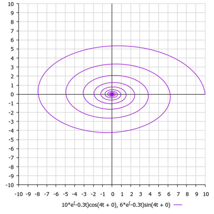
Figure 4. The value of the point along the Y coordinate is closer to the known value and its oscillation amplitude is smaller than that along the X axis

All plots on the graphs are made relative to zero, since we consider the difference relative to the value of the known optimum, that is, the displacement from zero is an increment.

Let's move on to the code description. First, let’s decide on the structure of the algorithm and create pseudocode:

1. Initialize point population
2. Calculate the fitness function value
3. Calculate the amplitude for each point coordinate when a new best optimum appears
4. When a new best optimum appears, "throw out" the best point in a random direction
   
5. Calculate the new position of the points using the equation of damped harmonic oscillations
6. Repeat from p. 2.

Point 4 was specially added and is intended to provide increased resistance to getting stuck, so that the points do not converge in a "spiral" to some local extremum and get stuck there. The authors of the algorithm do not cover this topic.

To describe an agent (particle, point), The S_Particle structure containing the following variables is well suited for describing the agent (particle, point):

• c  [] - array of particle coordinates
  
• cD[] - array of particle velocities
• t - iteration step, plays the role of "time" in the equation
  
• f - particle fitness function value
  

The structure also defines the Init function, which is used to initialize structure variables. The coords parameter specifies the number of particle coordinates.

//——————————————————————————————————————————————————————————————————————————————
struct S_Particle
{
  void Init (int coords)
  {
    ArrayResize (c,    coords);
    ArrayResize (cD,   coords);
    t = 0;
    f = -DBL_MAX;
  }

  double c  []; //coordinates
  double cD []; //coordinates
  int    t;     //iteration (time)
  double f;     //fitness
};
//——————————————————————————————————————————————————————————————————————————————

Let's define the SDOm algorithm class - C_AO_SDOm. The class contains the following variables and methods:

• cB [] - array of best coordinates
• fB - fitness function value of the best coordinates
• p [] - array of particles, data type - S_Particle
• rangeMax [] - array of maximum search range values
  
• rangeMin [] - array of minimum search range values
  
• rangeStep [] - array of search steps
  
• Init - method for initializing class parameters, accepts the following parameters: coordinatesNumberP - number of coordinates, populationSize - population size, dampingFactorP - damping ratio, frequencyP - frequency, precisionP - precision.
• Moving - method for moving particles in search space
• Revision - method for revising and updating the best coordinates
• coords - number of coordinates
• popSiz - population size
• A, e, γ, ω, φ - components of the damped harmonic oscillation equation
  
• precision, revision - private variables used inside the class
• SeInDiSp - calculate a new coordinate value in a given range with a given step
  
• RNDfromCI - method generates a random number in a given range

The code describes the C_AO_SDOm class, which represents an implementation of the algorithm with additional functions for revising and updating the best coordinates.

The first three variables of the class are the cB array, which stores the best coordinates, the fB variable, which stores the value of the fitness function of the best coordinates, and the p array, which stores the candidates (particles) of the population.

The next three class variables are rangeMax, rangeMin and rangeStep arrays, which store the maximum and minimum values of the search range and search steps, respectively.

Further on, the class contains three public methods: Init, Moving and Revision. Init is used to initialize class parameters and create an initial population of particles. Moving is used to move particles around the search space. Revision is applied to revise the best coordinates and update their values.

The class also contains several private variables used within the class. These are the coords and popSize variables, which store the number of coordinates and the population size, respectively. The A variable, which is used in the Moving method, the 'precision' variable, which stores the precision value, and the 'revision' variable, which is responsible for the need to revise the best coordinates.

The class contains several private methods: Research, SeInDiSp and RNDfromCI. Research is used to study new particle coordinates, while SeInDiSp and RNDfromCI are used to calculate random values in a given range.

“precision” is an external parameter of the algorithm, responsible for the discreteness of movement along the trajectory of a damped oscillation. The larger the value, the more accurately the trajectory is reproduced, and smaller values lead to "raggedness" of the trajectory (this does not mean that there will be a negative impact on the result, it depends on the task). The default setting was chosen as optimal after a series of my experiments.

//——————————————————————————————————————————————————————————————————————————————
class C_AO_SDOm
{
  //----------------------------------------------------------------------------
  public: double     cB []; //best coordinates
  public: double     fB;    //FF of the best coordinates
  public: S_Particle p  []; //particles

  public: double rangeMax  []; //maximum search range
  public: double rangeMin  []; //manimum search range
  public: double rangeStep []; //step search

  public: void Init (const int    coordinatesNumberP,   //coordinates number
                     const int    populationSizeP,      //population size
                     const double dampingFactorP,       //damping factor
                     const double frequencyP,           //frequency
                     const double precisionP);          //precision

  public: void Moving   ();
  public: void Revision ();

  //----------------------------------------------------------------------------
  private: int    coords;   //coordinates number
  private: int    popSize;  //population size

  private: double A;
  private: double e;
  private: double γ;
  private: double ω;
  private: double φ;
  private: double precision;

  private: bool   revision;

  private: double SeInDiSp  (double In, double InMin, double InMax, double Step);
  private: double RNDfromCI (double min, double max);
};
//——————————————————————————————————————————————————————————————————————————————

The Init method of the C_AO_SDOm class is used to initialize class parameters and create an initial population of particles.

First, MathSrand is used to reset the random number generator and the GetMicrosecondCount function is used to initialize the generator.

Next, the method sets initial values for the 'fB' and 'revision' variables, as well as assigns values to constant variables participating in the damped oscillation equation.

//——————————————————————————————————————————————————————————————————————————————
void C_AO_SDOm::Init (const int    coordinatesNumberP,   //coordinates number
                      const int    populationSizeP,      //population size
                      const double dampingFactorP,       //damping factor
                      const double frequencyP,           //frequency
                      const double precisionP)           //precision
{
  MathSrand ((int)GetMicrosecondCount ()); // reset of the generator
  fB       = -DBL_MAX;
  revision = false;

  coords  = coordinatesNumberP;
  popSize = populationSizeP;

  e = M_E;
  γ = dampingFactorP;
  ω = frequencyP;
  φ = 0.0;
  precision = precisionP;

  ArrayResize (rangeMax,  coords);
  ArrayResize (rangeMin,  coords);
  ArrayResize (rangeStep, coords);
  ArrayResize (cB,        coords);

  ArrayResize (p, popSize);

  for (int i = 0; i < popSize; i++)
  {
    p [i].Init (coords);
  }
}
//——————————————————————————————————————————————————————————————————————————————

We will use the Moving method to move particles in the search space.

The first code block (if (!revision)) is executed only on the first iteration and is intended to randomly place particles in the search space. The method then sets the value of 'revision' to 'true' so that the normal code block is used next time.

The next part of the method code is responsible for moving the population particles. If the fitness value of the current particle is equal to the fitness value of the best coordinates (p[i].f == fB), then the particle coordinates are updated in the same way as in the first code block. This means that the particle is thrown out of its position in a random direction to prevent all particles from converging on one single point.

Otherwise, the method uses the t variable to simulate the current time for each particle using the iteration counter (which is reset when the best global solution is updated). Then the coordinates of each particle are calculated using the equation of damped harmonic oscillations.

The commented out part of the code adds a random increment to the coordinate value calculated by the equation and can be used to create a beautiful visual fireworks effect. However, this effect has no practical value and does not improve the results, so the code is commented out.

//——————————————————————————————————————————————————————————————————————————————
void C_AO_SDOm::Moving ()
{
  //----------------------------------------------------------------------------
  if (!revision)
  {
    for (int i = 0; i < popSize; i++)
    {
      for (int c = 0; c < coords; c++)
      {
        p [i].c [c] = RNDfromCI (rangeMin [c], rangeMax [c]);
        p [i].c [c] = SeInDiSp (p [i].c [c], rangeMin [c], rangeMax [c], rangeStep [c]);
      }
    }

    revision = true;
    return;
  }

  //----------------------------------------------------------------------------
  int t = 0.0;

  for (int i = 0; i < popSize; i++)
  {
    if  (p [i].f == fB)
    {
      for (int c = 0; c < coords; c++)
      {
        p [i].c [c] = RNDfromCI (rangeMin [c], rangeMax [c]);
        p [i].c [c] = SeInDiSp (p [i].c [c], rangeMin [c], rangeMax [c], rangeStep [c]);
      }

      continue;
    }

    p [i].t++;
    t = p [i].t;

    for (int c = 0; c < coords; c++)
    {
      A = p [i].cD [c];
      φ = RNDfromCI (0.0, 2.0);

      p [i].c [c] = p [i].c [c] + A * pow (e, -γ * t / precision) * cos (ω * t / (precision) + φ);// + RNDfromCI (-0.01, 0.01) * (rangeMax [c] - rangeMin [c]);
      p [i].c [c] = SeInDiSp (p [i].c [c], rangeMin [c], rangeMax [c], rangeStep [c]);
    }
  }
}
//——————————————————————————————————————————————————————————————————————————————

The Revision class method is used to update the best coordinates and calculate the difference between the particle coordinates and the known best solution. This difference serves as the initial amplitude, and once a new better solution is found, the particles will begin to oscillate around the best known coordinates located at the center of these movements.

//——————————————————————————————————————————————————————————————————————————————
void C_AO_SDOm::Revision ()
{
  //----------------------------------------------------------------------------
  bool flag = false;
  for (int i = 0; i < popSize; i++)
  {
    if (p [i].f > fB)
    {
      flag = true;
      fB = p [i].f;
      ArrayCopy (cB, p [i].c, 0, 0, WHOLE_ARRAY);
    }
  }

  if (flag)
  {
    for (int i = 0; i < popSize; i++)
    {
      p [i].t = 0;

      for (int c = 0; c < coords; c++)
      {
        p [i].cD [c] = (cB [c] - p [i].c [c]);

      }
    }
  }
}
//——————————————————————————————————————————————————————————————————————————————

3. Test results

Test stand results seem to be good:

C_AO_SDOm:100;0.3;4.0;10000.0
=============================
5 Rastrigin's; Func runs 10000 result: 76.22736727464056
Score: 0.94450
25 Rastrigin's; Func runs 10000 result: 64.5695106264092
Score: 0.80005
500 Rastrigin's; Func runs 10000 result: 47.607500083305425
Score: 0.58988
=============================
5 Forest's; Func runs 10000 result: 1.3265635010116805
Score: 0.75037
25 Forest's; Func runs 10000 result: 0.5448141810532924
Score: 0.30817
500 Forest's; Func runs 10000 result: 0.12178250603909949
Score: 0.06889
=============================
5 Megacity's; Func runs 10000 result: 5.359999999999999
Score: 0.44667
25 Megacity's; Func runs 10000 result: 1.552
Score: 0.12933
500 Megacity's; Func runs 10000 result: 0.38160000000000005
Score: 0.03180
=============================
All score: 4.06967

Visualization of the SDOm algorithm revealed some distinctive features: the convergence graph for all test functions is unstable, the nature of the convergence curve changes throughout all iterations. This does not increase the feeling of confidence in the results. The Megacity function visualization specifically shows several repeated tests (usually only one is displayed in the video, so that the GIF would not turn out to be too big) to show the instability of the results from test to test. The spread of results is very large.

No features were noticed in the nature of the movement of particles, with the exception of the sharp Forest and discrete Megacity, where the coordinates of the particles line up in clearly visible lines. It is difficult to judge whether this is good or bad. For example, in the case of the ACOm algorithm it was a sign of qualitative convergence, but in the case of SDOm this is probably not the case.

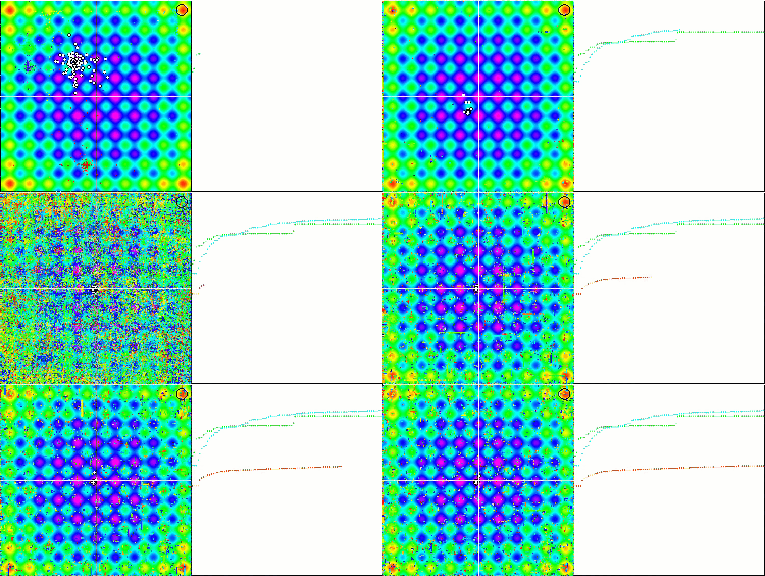
  SDOm on the Rastrigin test function.

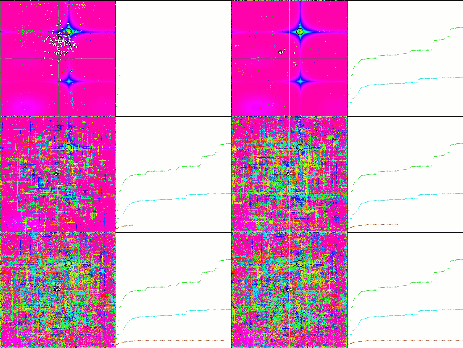
  SDOm on the Forest test function.

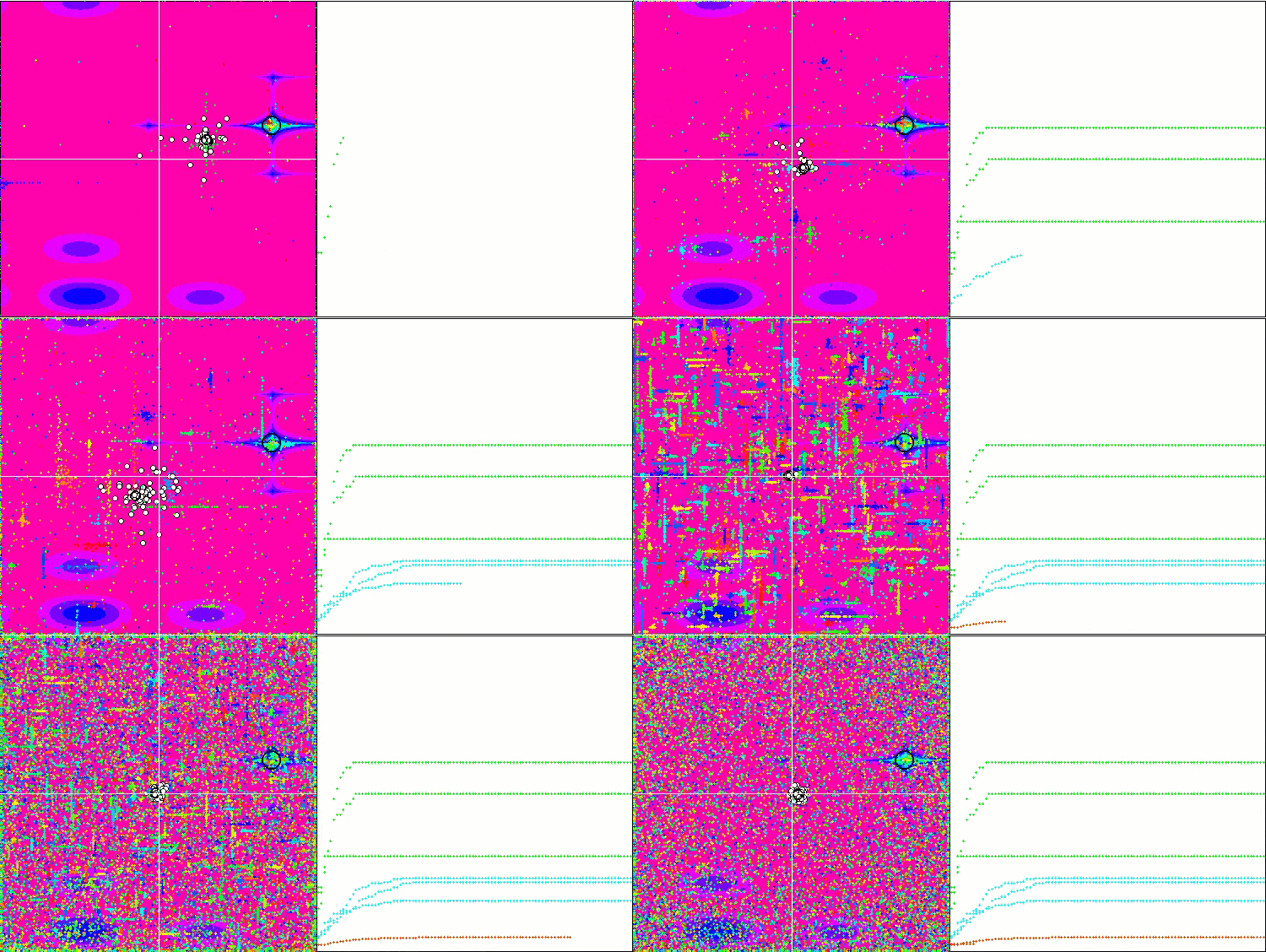
  SDOm on the Megacity test function.

When using the code commented out in the Moving method, which is responsible for adding random noise to the particle coordinate, an interesting phenomenon similar to fireworks occurs, while the random change in the phase of the oscillations is not used. I assume that after the mass convergence of particles to a known solution, they are ejected in different directions, and this is the reason for the beautiful effect demonstrating the moment the algorithm is stuck. This can be seen from the coincidence of the fireworks explosion with the beginning of the horizontal section of the convergence graph.

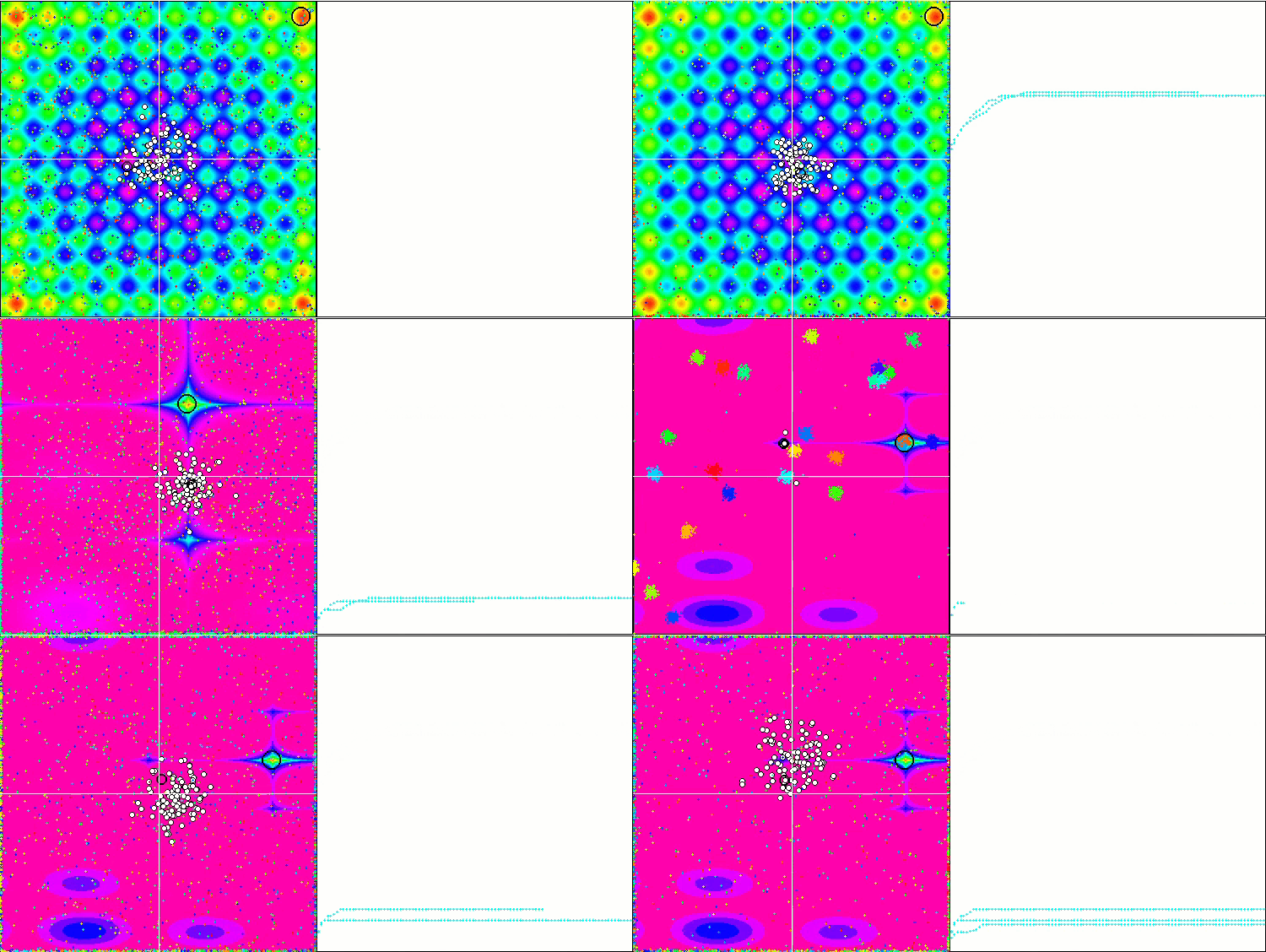
Demonstrating a useless but beautiful fireworks effect.

The SDOm algorithm has shown fairly good results overall and has been placed in the 8th place out of 23 participating in the rating table review. SDOm shows noticeably better results on the smooth Rastrigin function. The tendency to get stuck interferes with the results on the complex Forest and Megacity functions.

#	AO	Description	Rastrigin			Rastrigin final	Forest			Forest final	Megacity (discrete)			Megacity final	Final result
			10 p (5 F)	50 p (25 F)	1000 p (500 F)		10 p (5 F)	50 p (25 F)	1000 p (500 F)		10 p (5 F)	50 p (25 F)	1000 p (500 F)
1	SDSm	stochastic diffusion search M	0.99809	1.00000	0.69149	2.68958	1.00000	1.00000	1.00000	3.00000	1.00000	1.00000	1.00000	3.00000	100000
2	SDS	stochastic Diffusion Search	0.99737	0.97322	0.58904	2.55963	0.96778	0.93572	0.79649	2.69999	0.78696	0.93815	0.71804	2.44315	88.208
3	SSG	saplings sowing and growing	1.00000	0.92761	0.51630	2.44391	0.72654	0.65201	0.83760	2.21615	0.54782	0.61841	0.99522	2.16146	77.678
4	HS	harmony search	0.99676	0.88385	0.44686	2.32747	0.99882	0.68242	0.37529	2.05653	0.71739	0.71842	0.41338	1.84919	70.647
5	IWO	invasive weed optimization	0.95828	0.62227	0.27647	1.85703	0.70690	0.31972	0.26613	1.29275	0.57391	0.30527	0.33130	1.21048	48.267
6	ACOm	ant colony optimization M	0.34611	0.16683	0.15808	0.67103	0.86785	0.68980	0.64798	2.20563	0.71739	0.63947	0.05579	1.41265	47.419
7	MEC	mind evolutionary computation	0.99270	0.47345	0.21148	1.67763	0.60691	0.28046	0.21324	1.10061	0.66957	0.30000	0.26045	1.23002	44.061
8	SDOm	spiral dynamics optimization M	0.81076	0.56474	0.35334	1.72884	0.72333	0.30644	0.30985	1.33963	0.43479	0.13289	0.14695	0.71463	41.370
9	COAm	cuckoo optimization algorithm M	0.92400	0.43407	0.24120	1.59927	0.58309	0.23477	0.13842	0.95629	0.52174	0.24079	0.17001	0.93254	37.845
10	FAm	firefly algorithm M	0.59825	0.31520	0.15893	1.07239	0.51012	0.29178	0.41704	1.21894	0.24783	0.20526	0.35090	0.80398	33.152
11	ABC	artificial bee colony	0.78170	0.30347	0.19313	1.27829	0.53774	0.14799	0.11177	0.79750	0.40435	0.19474	0.13859	0.73768	29.784
12	BA	bat algorithm	0.40526	0.59145	0.78330	1.78002	0.20817	0.12056	0.21769	0.54641	0.21305	0.07632	0.17288	0.46225	29.488
13	CSS	charged system search	0.56605	0.68683	1.00000	2.25289	0.14065	0.01853	0.13638	0.29555	0.07392	0.00000	0.03465	0.10856	27.914
14	GSA	gravitational search algorithm	0.70167	0.41944	0.00000	1.12111	0.31623	0.25120	0.27812	0.84554	0.42609	0.25525	0.00000	0.68134	27.807
15	BFO	bacterial foraging optimization	0.67203	0.28721	0.10957	1.06881	0.39655	0.18364	0.17298	0.75317	0.37392	0.24211	0.18841	0.80444	27.549
16	EM	electroMagnetism-like algorithm	0.12235	0.42928	0.92752	1.47915	0.00000	0.02413	0.29215	0.31628	0.00000	0.00527	0.10872	0.11399	18.981
17	SFL	shuffled frog-leaping	0.40072	0.22021	0.24624	0.86717	0.20129	0.02861	0.02221	0.25211	0.19565	0.04474	0.06607	0.30646	13.201
18	MA	monkey algorithm	0.33192	0.31029	0.13582	0.77804	0.10000	0.05443	0.07482	0.22926	0.15652	0.03553	0.10669	0.29874	11.771
19	FSS	fish school search	0.46812	0.23502	0.10483	0.80798	0.12825	0.03458	0.05458	0.21741	0.12175	0.03947	0.08244	0.24366	11.329
20	IWDm	intelligent water drops M	0.26459	0.13013	0.07500	0.46972	0.28568	0.05445	0.05112	0.39126	0.22609	0.05659	0.05054	0.33322	10.434
21	PSO	particle swarm optimisation	0.20449	0.07607	0.06641	0.34696	0.18873	0.07233	0.18207	0.44313	0.16956	0.04737	0.01947	0.23641	8.431
22	RND	random	0.16826	0.09038	0.07438	0.33302	0.13480	0.03318	0.03949	0.20747	0.12175	0.03290	0.04898	0.20363	5.056
23	GWO	grey wolf optimizer	0.00000	0.00000	0.02093	0.02093	0.06562	0.00000	0.00000	0.06562	0.23478	0.05789	0.02545	0.31812	1.000

Summary

The original approach to the implementation of the modified version made it possible to avoid heavy matrix calculations as in the original author's algorithm, and also made it possible to make it universal without reference to the relationships between coordinates for n-dimensional space.

I have made attempts to use the concept of "mass" in the equation for damped harmonic oscillations in order to make the behavior of particles individual depending on their fitness. The idea was to reduce the amplitude and frequency of particles with a larger mass (with a better value of the fitness function), while lighter particles would have to make movements that were larger in amplitude and with a higher frequency. This could provide a higher degree of refinement of the known best solutions, while at the same time increasing search capabilities due to the "broad" motions of light particles. Unfortunately, this idea did not bring the expected improvement in results.

Physical simulation of particle trajectories in the algorithm suggests the possibility of using such physical concepts as speed, acceleration and inertia. This is a matter of further research.

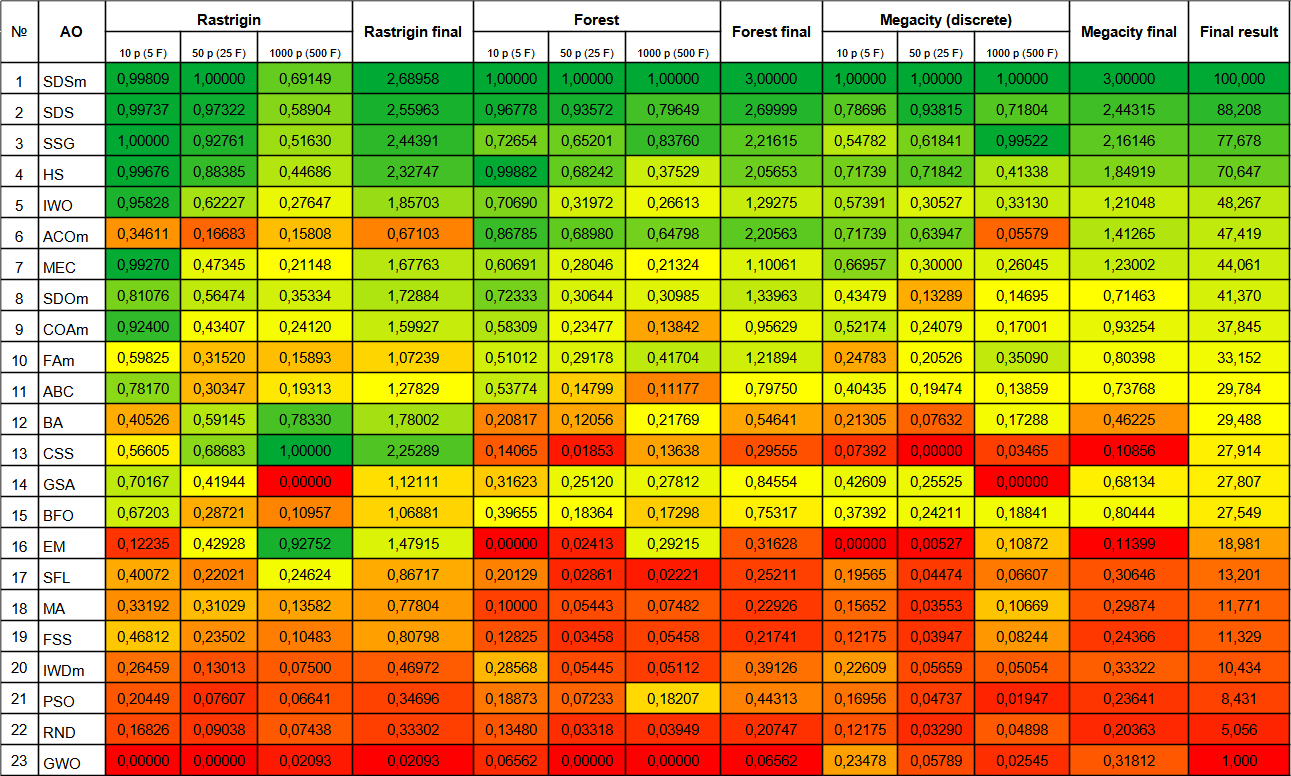
Figure 5. Color gradation of algorithms according to relevant tests

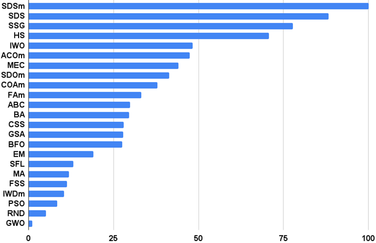
Figure 6. The histogram of algorithm test results (on a scale from 0 to 100, the more the better,

the archive contains the script for calculating the rating table using the method applied in the article).

Pros and cons of the modified Spiral Dynamics Optimization (SDOm) algorithm:

Pros:
1. A small number of external parameters.
2. Simple implementation.
3. Operation speed.

Cons:
1. High scatter of results.
2. Tendency to get stuck in local extremes.

The article is accompanied by an archive with updated current versions of the algorithm codes described in previous articles. The author of the article is not responsible for the absolute accuracy in the description of canonical algorithms. Changes have been made to many of them to improve search capabilities. The conclusions and judgments presented in the articles are based on the results of the experiments.