Population optimization algorithms: Bat algorithm (BA)

Contents

1. Introduction
2. Algorithm description
3. Test results

1. Introduction

Bats are amazing animals. Scientists believe that the first bats appeared 65-100 million years ago living side by side with dinosaurs. Bats are the only winged mammals. The bats boast over 1300 species. They can be found almost everywhere except the polar regions. During the day, they hide in shelters. To navigate dark caves and hunt after dark, bats rely on echolocation, a system that allows them to detect objects using sound waves. They echolocate by emitting a high frequency sound that moves forward until it hits an object and is reflected back. Echolocation is a kind of sonar: a bat emits a loud and short pulsed sound. When the sound reaches an object, the echo returns to the bat's ears after a short period of time, which is how bats orient themselves in space and determine the position of their prey. 

The Bat Algorithm (BA) is a heuristic algorithm introduced by Yang in 2010 that mimics the echolocation behavior of bats to perform global optimization. Metaheuristics, usually inspired by nature and physical processes, is now used as one of the most powerful techniques for solving many complex optimization problems. Optimization is the selection of the best elements for a certain set of criteria from a number of efficient options, which shows many different advantages and disadvantages in terms of computational efficiency and the likelihood of global optimization.

Feature optimization offers a formal framework for modeling and solving a number of specific problems by providing a "target" function that takes a parameter as an input. The goal is to find the value of the combined parameter to return the best value. This framework is abstract enough so that various problems can be interpreted as "feature optimization" problems.

However, traditional feature optimization is used only to solve some small problems, which are often not applicable in practice. Therefore, scientists are turning their attention to nature, which provides rich models for solving these problems. By modeling natural biological systems, many intelligent swarm optimization algorithms are proposed for solving applied problems using unconventional methods. They are widely used in various optimization problems due to their excellent performance. BA is a new and modern swarm-like algorithm that performs a search process using artificial bats as search agents simulating the natural sound pulse volume and emission frequency of real bats.

2. Algorithm description

In the basic bat algorithm, each bat is treated as a "massless and sizeless" particle representing a valid solution in the solution space. For different fitness functions, each bat has a corresponding feature value and determines the current optimal individual by comparing the feature values. Then the frequency of the acoustic wave, the speed, the speed of the emission of impulses and the volume of each bat in the population are updated, iterative evolution continues, the current optimal solution is approximated and generated, and finally the global optimal solution is found. The algorithm updates the frequency, speed and position of each bat.

The standard algorithm requires five basic parameters: frequency, loudness, ripple, and loudness and ripple ratios. The frequency is used to balance the impact of the historical best position on the current position. An individual bat will search far from the group's historical position when the search frequency range is large, and vice versa.

There are quite a lot of parameters of the algorithm compared to the ones considered earlier:

input double MIN_FREQ_P          = 0.0;
input double MAX_FREQ_P         = 1.0;
input double MIN_LOUDNESS_P  = 0.0;
input double MAX_LOUDNESS_P = 1.5;
input double MIN_PULSE_P        = 0.0;
input double MAX_PULSE_P        = 1.0;
input double ALPHA_P               = 0.3;
input double GAMMA_P              = 0.3;

When implementing the BA algorithm, I came across the fact that in many sources the authors of the articles describe the algorithm in completely different ways. The differences are both in the use of terms in the description of key points and in the fundamental algorithmic features, so I will describe how I understood it myself. The basic physical principles underlying echolocation can be applied in the algorithm with significant reservations and conventions. We assume that the bats use sound pulses with the frequency ranging from MinFreq to MaxFreq. The frequency affects the bat velocity. The conditional concept of loudness is also used, which affects the transition from the state of local search at the location of the current position of the bat to the global one in the vicinity of the best solution. The pulsation frequency increases throughout the optimization, while the volume of the sounds decreases.

BA algorithm pseudo code (Fig. 1):

1. Bat population initialization.
2. Generation of frequency, speed and new solutions.
3. Search for a local solution.
4. Updating the global solution.
5. Decreasing the volume and increasing the pulsation frequency.
6. Repeat step 2 until the stop criterion is met.

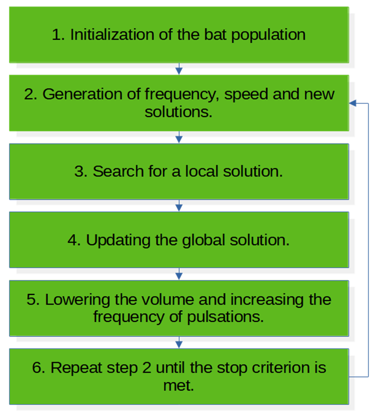
Fig. 1. BA algorithm block diagram

Let's start describing the code. To describe the "bat" search agent, we need a structure in which we describe all the characteristics necessary for a complete description of the state at the time of each iteration. The position [] array is used to store the best position coordinates in space, while the auxPosition [] array is for the current "operational" coordinates. The speed [] array is needed in the calculation of the velocity vector by coordinates. frequency - frequency of sound pulses, initPulseRate - initial pulse rate (individual for each bat from the very beginning of optimization), pulseRate - pulse rate at the current iteration, loudness - loudness of sound pulses, fitness - fitness function value after the last move, fitnessBest - best value of the agent's fitness function for all iterations. 

//——————————————————————————————————————————————————————————————————————————————
struct S_Bat
{
  double position    [];
  double auxPosition [];
  double speed       [];
  double frequency;
  double initPulseRate;
  double pulseRate;
  double loudness;
  double fitness;
  double fitnessBest;
};
//——————————————————————————————————————————————————————————————————————————————

The bat algorithm class includes an array of structures of search agents, boundaries and step of the explored space, the best coordinates found by the algorithm, the best value of the fitness function and constants for storing algorithm parameters, as well as the public initialization method, two public methods required for operation with the algorithm and algorithm-specific private methods.

//——————————————————————————————————————————————————————————————————————————————
class C_AO_BA
{
  //============================================================================
  public: S_Bat  bats      []; //bats
  public: double rangeMax  []; //maximum search range
  public: double rangeMin  []; //manimum search range
  public: double rangeStep []; //step search
  public: double cB        []; //best coordinates
  public: double fB;           //FF of the best coordinates

  public: void Init (const int    paramsP,
                     const int    batsNumberP,
                     const double min_FREQ_P,
                     const double max_FREQ_P,
                     const double min_LOUDNESS_P,
                     const double max_LOUDNESS_P,
                     const double min_PULSE_P,
                     const double max_PULSE_P,
                     const double alpha_P,
                     const double gamma_P,
                     const int    maxIterP);

  public: void Flight (int epoch);
  public: void Preparation ();

  //============================================================================
  private: void Walk               (S_Bat &bat);
  private: void AproxBest          (S_Bat &bat, double averageLoudness);
  private: void AcceptNewSolutions (S_Bat &bat);
  private: int  currentIteration;
  private: int  maxIter;

  private: double MIN_FREQ;
  private: double MAX_FREQ;

  private: double MIN_LOUDNESS;
  private: double MAX_LOUDNESS;

  private: double MIN_PULSE;
  private: double MAX_PULSE;

  private: double ALPHA;
  private: double GAMMA;

  private: int    params;
  private: int    batsNumber;

  private: bool   firstFlight;

  private: double SeInDiSp  (double In, double inMin, double inMax, double step);
  private: double RNDfromCI (double min, double max);
  private: double Scale     (double In, double InMIN, double InMAX, double OutMIN, double OutMAX,  bool revers);
};
//——————————————————————————————————————————————————————————————————————————————

In the Init () public method of the algorithm setting parameters, allocate the memory for arrays, reset the variable to the minimum value to store the best fit and reset the flag of the initial iteration. In general, this method is not complicated and something special.

//——————————————————————————————————————————————————————————————————————————————
void C_AO_BA::Init (const int    paramsP,
                    const int    batsNumberP,
                    const double min_FREQ_P,
                    const double max_FREQ_P,
                    const double min_LOUDNESS_P,
                    const double max_LOUDNESS_P,
                    const double min_PULSE_P,
                    const double max_PULSE_P,
                    const double alpha_P,
                    const double gamma_P,
                    const int    maxIterP)
{
  MathSrand (GetTickCount ());

  fB = -DBL_MAX;

  params       = paramsP;
  batsNumber   = batsNumberP;
  MIN_FREQ     = min_FREQ_P;
  MAX_FREQ     = max_FREQ_P;
  MIN_LOUDNESS = min_LOUDNESS_P;
  MAX_LOUDNESS = max_LOUDNESS_P;
  MIN_PULSE    = min_PULSE_P;
  MAX_PULSE    = max_PULSE_P;
  ALPHA        = alpha_P;
  GAMMA        = gamma_P;
  maxIter      = maxIterP;

  ArrayResize (rangeMax,  params);
  ArrayResize (rangeMin,  params);
  ArrayResize (rangeStep, params);

  firstFlight = false;

  ArrayResize (bats, batsNumber);

  for (int i = 0; i < batsNumber; i++)
  {
    ArrayResize (bats [i].position,    params);
    ArrayResize (bats [i].auxPosition, params);
    ArrayResize (bats [i].speed,       params);

    bats [i].fitness  = -DBL_MAX;
  }

  ArrayResize (cB, params);
}
//——————————————————————————————————————————————————————————————————————————————

The first method called on each iteration is Flight(). It concentrates the main frame of the search logic, and the rest of the details are placed in auxiliary private methods specific to this optimization algorithm. At the very first iteration, the firstFlight flag is reset (the reset occurs during initialization in the Init () method).This means that we need to assign an initial state to each bat, which is a random position in the search space:

• zero speed,
• individual frequency of sound pulses assigned by a random number in the range specified by the parameters,
• initial individual pulsation frequency also defined by a random number in the parameter range
• and the loudness of sound pulses in the parameter range.

As you can see, each artificial bat has an individual set of characteristics of sound signals, which makes them more like real bats in nature. In the entire population, which may consist of several hundred thousand individuals, a mother can find one single cub by the unique sound signature the baby emits.

If the firstFlight flag is enabled, then it is necessary to carry out basic operations to move bats. One of the interesting features of the algorithm lies in the concept of the average sound loudness of the entire population. In general, the sound loudness decreases via the 'alpha' coefficient throughout all iterations. There are two types of bat movement here: Walk () - individual movement with the calculation of the velocity vector for each coordinate component and local movement in the vicinity of the best solution.

With each next iteration, the intensity of pulsations decreases, which affects the intensity of the neighborhood exploration. Thus, exploration and exploitation change dynamically throughout the optimization. Next, we will see how the current iteration affects the behavior of bats.

//——————————————————————————————————————————————————————————————————————————————
void C_AO_BA::Flight (int epoch)
{
  currentIteration = epoch;

  //============================================================================
  if (!firstFlight)
  {
    fB = -DBL_MAX;

    //--------------------------------------------------------------------------
    for (int b = 0; b < batsNumber; b++)
    {
      for (int p = 0; p < params; p++)
      {
        bats [b].position    [p] = RNDfromCI (rangeMin [p], rangeMax [p]);
        bats [b].position    [p] = SeInDiSp (bats [b].position [p], rangeMin [p], rangeMax [p], rangeStep [p]);
        bats [b].auxPosition [p] = bats [b].position    [p];
        bats [b].speed       [p] = 0.0;
        bats [b].frequency       = RNDfromCI (MIN_FREQ, MAX_FREQ);
        bats [b].initPulseRate   = RNDfromCI (MIN_PULSE, MAX_PULSE / 2);
        bats [b].pulseRate       = bats [b].initPulseRate;
        bats [b].loudness        = RNDfromCI (MAX_LOUDNESS / 2, MAX_LOUDNESS);
        bats [b].fitness         = -DBL_MAX;
        bats [b].fitnessBest     = -DBL_MAX;
      }
    }

    firstFlight = true;
  }
  //============================================================================
  else
  {
    double avgLoudness = 0;

    for (int b = 0; b < batsNumber; b++)
    {
      avgLoudness += bats [b].loudness;
    }

    avgLoudness /= batsNumber;

    for (int b = 0; b < batsNumber; b++)
    {
      Walk (bats [b]);

      if (RNDfromCI (MIN_PULSE, MAX_PULSE) > bats [b].pulseRate)
      {
        AproxBest (bats [b], avgLoudness);
      }
    }
  }
}
//——————————————————————————————————————————————————————————————————————————————

The second required public method called on each iteration - Preparation() is needed to update the global best solution. Here we can see how the concept of "loudness" is used. Since with each iteration the volume of each mouse decreases through a factor ('alpha' algorithm tuning parameter), the probability of a local study decreases together with the intensity of the global solution study. In other words, the probability of updating the best position of each bat decreases with each iteration. This is one of those moments in the algorithm that is the least understood, at least for me. However, the author of the algorithm implemented this, which means it is necessary.

//——————————————————————————————————————————————————————————————————————————————
void C_AO_BA::Preparation ()
{
  //----------------------------------------------------------------------------
  for (int b = 0; b < batsNumber; b++)
  {
    if (bats [b].fitness > fB)
    {
      fB = bats [b].fitness;
      ArrayCopy (cB, bats [b].auxPosition, 0, 0, WHOLE_ARRAY);
    }
  }

  //----------------------------------------------------------------------------
  for (int b = 0; b < batsNumber; b++)
  {
    if (RNDfromCI (MIN_LOUDNESS, MAX_LOUDNESS) < bats [b].loudness && bats [b].fitness >= bats [b].fitnessBest)
    {
      AcceptNewSolutions (bats [b]);
    }
  }
}
//——————————————————————————————————————————————————————————————————————————————

The private Walk() method ensures that each bat moves individually relative to its current best position so far, given the global best solution. This method uses the frequency of sound pulses, which varies randomly within the [MIN_FREQ;MAX_FREQ] range. The frequency is needed to calculate the speed of movement of the search agent, which is the product of the frequency by the difference between the best mouse position and the best global solution. After that, the speed value is added to the current best solution of the bat vector by vector. Thus, we operate with disproportionate physical quantities, but what can we do? This is only an approximation to real physical objects. Plausibility has to be neglected in this case. After calculating the new position, the coordinates should be checked for out-of-range using the SeInDiSp () method.

//——————————————————————————————————————————————————————————————————————————————
void C_AO_BA::Walk (S_Bat &bat)
{
  for (int j = 0; j < params; ++j)
  {
    bat.frequency       = MIN_FREQ + (MAX_FREQ - MIN_FREQ) * RNDfromCI (0.0, 1.0);
    bat.speed       [j] = bat.speed [j] + (bat.position [j] - cB [j]) * bat.frequency;
    bat.auxPosition [j] = bat.position [j] + bat.speed [j];

    bat.auxPosition [j] = SeInDiSp (bat.auxPosition [j], rangeMin [j], rangeMax [j], rangeStep [j]);
  }
}
//——————————————————————————————————————————————————————————————————————————————

The second private method, AproxBest(), is responsible for moving the bats relative to the global best solution providing additional coordinate refinement. It is not possible for me to understand the physical meaning of this action, which consists in the vector-by-vector addition to the coordinates of the increment in the form of the average loudness among the entire population of bats multiplied by a random number in the [-1.0; 1.0] range. I tried to reduce the values to the dimension of the function being optimized through the vector of valid values of the definition domain, but the test results turned out to be worse than in the author's version of the algorithm, so I left everything as it is, but I am sure that the efficiency of the BA algorithm can be improved, but this will require additional research, which was not the goal in this case. After calculating the coordinates, the values are checked for out-of-range using the SeInDiSp () method.

//——————————————————————————————————————————————————————————————————————————————
void C_AO_BA::AproxBest (S_Bat &bat, double averageLoudness)
{
  for (int j = 0; j < params; ++j)
  {
    bat.auxPosition [j] = cB [j] + averageLoudness * RNDfromCI (-1.0, 1.0);
    bat.auxPosition [j] = SeInDiSp (bat.auxPosition [j], rangeMin [j], rangeMax [j], rangeStep [j]);
  }
}
//——————————————————————————————————————————————————————————————————————————————

Another specific private method is AcceptNewSolutions (), which is called when the test condition for the frequency of the sound pulses for each bat is met. The new best individual solution is accepted, as well as the individual loudness and the individual pulsation frequency are recalculated here. Here we can see how the ordinal number of an iteration is involved in the calculation of the pulsation frequency.

At this point in the logic of the algorithm, I took some liberties and changed the logic, making the result independent of the dimension of the total number of iterations, which ultimately slightly increased the efficiency of the algorithm. In the original version, the iteration number was directly involved in the non-linear formula for calculating the pulse frequency. BA already features a lot of conventions. I could not close my eyes to one more in this case.

//——————————————————————————————————————————————————————————————————————————————
void C_AO_BA::AcceptNewSolutions (S_Bat &bat)
{
  ArrayCopy(bat.position, bat.auxPosition, 0, 0, WHOLE_ARRAY);
  bat.fitnessBest = bat.fitness;
  bat.loudness    = ALPHA * bat.loudness;
  double iter     = Scale (currentIteration, 1, maxIter, 0.0, 10.0, false);
  bat.pulseRate   = bat.initPulseRate *(1.0 - exp(-GAMMA * iter));
}
//——————————————————————————————————————————————————————————————————————————————

The dependence of the pulsation frequency on the number of the current iteration (x on the graph) and the GAMMA setting parameter is shown in Figure 2.

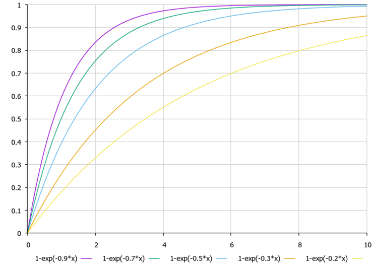
Fig 2. Dependence of the pulsation frequency on the number of the current iteration and the GAMMA setting parameter with the values of 0.9, 0.7, 0.5, 0.3, 0.2

3. Test results

In the last article, I mentioned plans to revise the methodology for calculating the rating of tested algorithms. First, since most algorithms can easily cope with the test functions of two variables and the difference between the results is almost indistinguishable, I decided to increase the number of variables for the first two tests on all test functions. Now the number of variables will be 10, 50 and 1000.

Second, the Skin test function has been replaced with the widely used Rastrigin function (Figure 3). This function is smooth like Skin. It has a complex surface with many local extrema, a global maximum at four points and one global minimum at the center of the coordinate axes.

Thirdly, I decided to normalize the test results to a range of values among all the algorithms in the table, where the best result is 1.0, and the worst result is 0.0. This allows us to evenly evaluate the test results, while the complexity of the functions is taken into account according to the results of each of the optimization algorithms in testing.

After that, the results of testing the algorithms are summed up. The maximum result is assigned a value of 100 (reference maximum result), while the minimum value is 1. This allows us to directly compare the algorithms with each other evenly considering the complexity of the test functions. Now the results printed in Print () are saved in the source files of the test scripts for each algorithm, respectively. The script that calculates the scores in the tests is attached below. It will be updated in subsequent articles with the addition of the results of the new algorithms under consideration.

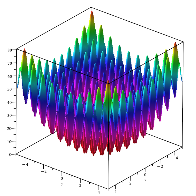
Fig. 3. Rastrigin test function

The test stand results look as follows:

2022.12.28 17:13:46.384    Test_AO_BA (EURUSD,M1)    C_AO_BA:50;0.0;1.0;0.0;1.5;0.0;1.0;0.3;0.3
2022.12.28 17:13:46.384    Test_AO_BA (EURUSD,M1)    =============================
2022.12.28 17:13:48.451    Test_AO_BA (EURUSD,M1)    5 Rastrigin's; Func runs 10000 result: 66.63334336098077
2022.12.28 17:13:48.451    Test_AO_BA (EURUSD,M1)    Score: 0.82562
2022.12.28 17:13:52.630    Test_AO_BA (EURUSD,M1)    25 Rastrigin's; Func runs 10000 result: 65.51391114042588
2022.12.28 17:13:52.630    Test_AO_BA (EURUSD,M1)    Score: 0.81175
2022.12.28 17:14:27.234    Test_AO_BA (EURUSD,M1)    500 Rastrigin's; Func runs 10000 result: 59.84512760590815
2022.12.28 17:14:27.234    Test_AO_BA (EURUSD,M1)    Score: 0.74151
2022.12.28 17:14:27.234    Test_AO_BA (EURUSD,M1)    =============================
2022.12.28 17:14:32.280    Test_AO_BA (EURUSD,M1)    5 Forest's; Func runs 10000 result: 0.5861602092218606
2022.12.28 17:14:32.280    Test_AO_BA (EURUSD,M1)    Score: 0.33156
2022.12.28 17:14:39.204    Test_AO_BA (EURUSD,M1)    25 Forest's; Func runs 10000 result: 0.2895682720055589
2022.12.28 17:14:39.204    Test_AO_BA (EURUSD,M1)    Score: 0.16379
2022.12.28 17:15:14.716    Test_AO_BA (EURUSD,M1)    500 Forest's; Func runs 10000 result: 0.09867854051596259
2022.12.28 17:15:14.716    Test_AO_BA (EURUSD,M1)    Score: 0.05582
2022.12.28 17:15:14.716    Test_AO_BA (EURUSD,M1)    =============================
2022.12.28 17:15:20.843    Test_AO_BA (EURUSD,M1)    5 Megacity's; Func runs 10000 result: 3.3199999999999994
2022.12.28 17:15:20.843    Test_AO_BA (EURUSD,M1)    Score: 0.27667
2022.12.28 17:15:26.624    Test_AO_BA (EURUSD,M1)    25 Megacity's; Func runs 10000 result: 1.2079999999999997
2022.12.28 17:15:26.624    Test_AO_BA (EURUSD,M1)    Score: 0.10067
2022.12.28 17:16:05.013    Test_AO_BA (EURUSD,M1)    500 Megacity's; Func runs 10000 result: 0.40759999999999996
2022.12.28 17:16:05.013    Test_AO_BA (EURUSD,M1)    Score: 0.03397

The bat algorithm has shown impressive results on the smooth Rastrigin function. Interestingly, with an increase in the number of variables in the function, the stability (repeatability) of the results increases, which indicates excellent scalability of BA on smooth functions. In particular, BA turned out to be the best on the Rastrigin function with 50 and 1000 variables among all test participants, which allows us to recommend the bat algorithm for working with complex smooth functions and neural networks. On the Forest and Megacity functions, the bat algorithm showed average results demonstrating a tendency to get stuck in local extremes. The coordinates are localized into groups and do not show the dynamics of change and movement towards the global optimum. I think, this happens because the algorithm is sensitive to the presence of a gradient on the surface of the function under study. In the absence of the gradient, the algorithm quickly stops in the vicinity of local areas that do not have a significant increment in the fitness function values. Moreover, the BA algorithm lacks mechanisms that allow "jumping" to new unknown areas, similar to the mechanism implemented in COA (Levy flights).

I should also mention a large number of settings for BA. Not only are there many parameters (degrees of freedom), but each of them greatly affects both the nature of the search properties and the overall convergence rates. Some parameters can give excellent results on smooth functions, and some on discrete and fissure functions. Finding some universal parameters that make it possible to cope equally well with different types of test functions is a difficult task. The article features the source code of the bat algorithm with the parameters that seem the most optimal to me. In general, I would not recommend using BA for users who have little experience in working with optimization algorithms, since optimization results can vary greatly.  

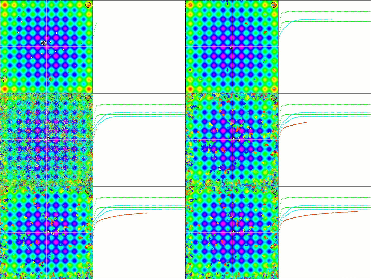
  BA on the Rastrigin test function

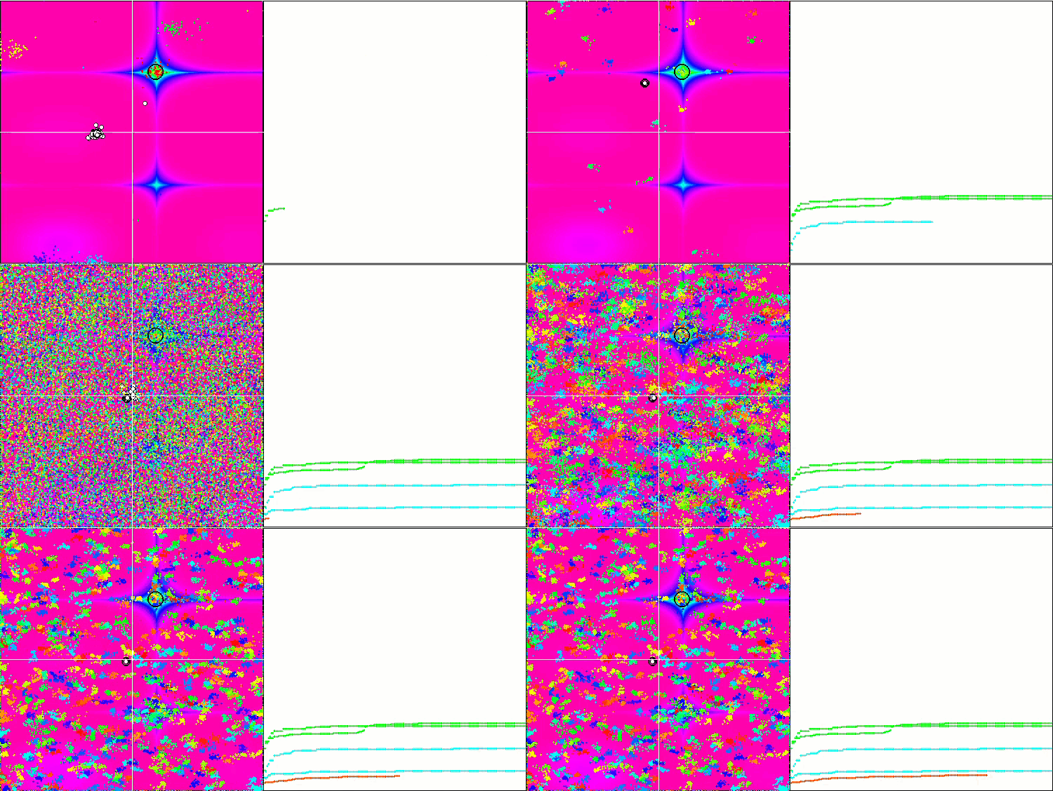
BA on the Forest test function

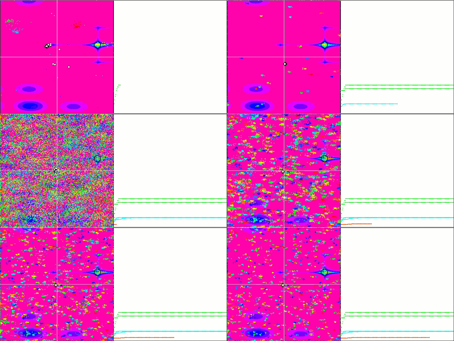
BA on the Megacity test function

While focusing on the visualization of test functions, one can get an idea of the characteristic features of the bat algorithm. In particular, when working on all test functions, the algorithm is characterized by grouping coordinates in very small local areas. While for a smooth function this feature makes it possible to move even where the gradient of the fitness function changes slightly, on a discrete function this feature proves to be a disadvantage since the algorithm gets stuck on flat plateaus.

Results obtained by the script calculating the scores of the optimization algorithms:

2023.01.03 17:55:57.386    CalculationTestResults (EURUSD,M1)    =======C_AO_RND=======
2023.01.03 17:55:57.386    CalculationTestResults (EURUSD,M1)    0.18210 | 0.15281 | 0.07011 |
2023.01.03 17:55:57.386    CalculationTestResults (EURUSD,M1)    0.08623 | 0.04810 | 0.06094 |
2023.01.03 17:55:57.386    CalculationTestResults (EURUSD,M1)    0.00000 | 0.00000 | 0.08904 |
2023.01.03 17:55:57.386    CalculationTestResults (EURUSD,M1)    0.6893397068905002
2023.01.03 17:55:57.386    CalculationTestResults (EURUSD,M1)    =======C_AO_PSO=======
2023.01.03 17:55:57.386    CalculationTestResults (EURUSD,M1)    0.22131 | 0.12861 | 0.05966 |
2023.01.03 17:55:57.386    CalculationTestResults (EURUSD,M1)    0.15345 | 0.10486 | 0.28099 |
2023.01.03 17:55:57.386    CalculationTestResults (EURUSD,M1)    0.08028 | 0.02385 | 0.00000 |
2023.01.03 17:55:57.386    CalculationTestResults (EURUSD,M1)    1.053004072893302
2023.01.03 17:55:57.386    CalculationTestResults (EURUSD,M1)    =======C_AO_ACOm=======
2023.01.03 17:55:57.386    CalculationTestResults (EURUSD,M1)    0.37458 | 0.28208 | 0.17991 |
2023.01.03 17:55:57.386    CalculationTestResults (EURUSD,M1)    1.00000 | 1.00000 | 1.00000 |
2023.01.03 17:55:57.386    CalculationTestResults (EURUSD,M1)    1.00000 | 1.00000 | 0.10959 |
2023.01.03 17:55:57.386    CalculationTestResults (EURUSD,M1)    5.946151922377553
2023.01.03 17:55:57.386    CalculationTestResults (EURUSD,M1)    =======C_AO_ABC=======
2023.01.03 17:55:57.386    CalculationTestResults (EURUSD,M1)    0.84599 | 0.51308 | 0.22588 |
2023.01.03 17:55:57.386    CalculationTestResults (EURUSD,M1)    0.58850 | 0.21455 | 0.17249 |
2023.01.03 17:55:57.386    CalculationTestResults (EURUSD,M1)    0.47444 | 0.26681 | 0.35941 |
2023.01.03 17:55:57.386    CalculationTestResults (EURUSD,M1)    3.661160435265267
2023.01.03 17:55:57.386    CalculationTestResults (EURUSD,M1)    =======C_AO_GWO=======
2023.01.03 17:55:57.386    CalculationTestResults (EURUSD,M1)    0.00000 | 0.00000 | 0.00000 |
2023.01.03 17:55:57.386    CalculationTestResults (EURUSD,M1)    0.00000 | 0.00000 | 0.00000 |
2023.01.03 17:55:57.386    CalculationTestResults (EURUSD,M1)    0.18977 | 0.04119 | 0.01802 |
2023.01.03 17:55:57.386    CalculationTestResults (EURUSD,M1)    0.24898721240154956
2023.01.03 17:55:57.386    CalculationTestResults (EURUSD,M1)    =======C_AO_COAm=======
2023.01.03 17:55:57.386    CalculationTestResults (EURUSD,M1)    1.00000 | 0.73390 | 0.28892 |
2023.01.03 17:55:57.386    CalculationTestResults (EURUSD,M1)    0.64504 | 0.34034 | 0.21362 |
2023.01.03 17:55:57.386    CalculationTestResults (EURUSD,M1)    0.67153 | 0.34273 | 0.45422 |
2023.01.03 17:55:57.386    CalculationTestResults (EURUSD,M1)    4.690306586791184
2023.01.03 17:55:57.386    CalculationTestResults (EURUSD,M1)    =======C_AO_FSS=======
2023.01.03 17:55:57.386    CalculationTestResults (EURUSD,M1)    0.50663 | 0.39737 | 0.11006 |
2023.01.03 17:55:57.386    CalculationTestResults (EURUSD,M1)    0.07806 | 0.05013 | 0.08423 |
2023.01.03 17:55:57.386    CalculationTestResults (EURUSD,M1)    0.00000 | 0.01084 | 0.18998 |
2023.01.03 17:55:57.386    CalculationTestResults (EURUSD,M1)    1.4272897567648186
2023.01.03 17:55:57.386    CalculationTestResults (EURUSD,M1)    =======C_AO_FAm=======
2023.01.03 17:55:57.386    CalculationTestResults (EURUSD,M1)    0.64746 | 0.53292 | 0.18102 |
2023.01.03 17:55:57.386    CalculationTestResults (EURUSD,M1)    0.55408 | 0.42299 | 0.64360 |
2023.01.03 17:55:57.386    CalculationTestResults (EURUSD,M1)    0.21167 | 0.28416 | 1.00000 |
2023.01.03 17:55:57.386    CalculationTestResults (EURUSD,M1)    4.477897116029613
2023.01.03 17:55:57.386    CalculationTestResults (EURUSD,M1)    =======C_AO_BA=======
2023.01.03 17:55:57.386    CalculationTestResults (EURUSD,M1)    0.43859 | 1.00000 | 1.00000 |
2023.01.03 17:55:57.386    CalculationTestResults (EURUSD,M1)    0.17768 | 0.17477 | 0.33595 |
2023.01.03 17:55:57.386    CalculationTestResults (EURUSD,M1)    0.15329 | 0.07158 | 0.46287 |
2023.01.03 17:55:57.386    CalculationTestResults (EURUSD,M1)    3.8147314003892507
2023.01.03 17:55:57.386    CalculationTestResults (EURUSD,M1)    ================
2023.01.03 17:55:57.386    CalculationTestResults (EURUSD,M1)    ================
2023.01.03 17:55:57.386    CalculationTestResults (EURUSD,M1)    ================
2023.01.03 17:55:57.386    CalculationTestResults (EURUSD,M1)    0.24898721240154956 | 5.946151922377553
2023.01.03 17:55:57.386    CalculationTestResults (EURUSD,M1)    C_AO_RND: 8.652
2023.01.03 17:55:57.386    CalculationTestResults (EURUSD,M1)    C_AO_PSO: 14.971
2023.01.03 17:55:57.386    CalculationTestResults (EURUSD,M1)    C_AO_ACOm: 100.000
2023.01.03 17:55:57.386    CalculationTestResults (EURUSD,M1)    C_AO_ABC: 60.294
2023.01.03 17:55:57.386    CalculationTestResults (EURUSD,M1)    C_AO_GWO: 1.000
2023.01.03 17:55:57.386    CalculationTestResults (EURUSD,M1)    C_AO_COAm: 78.177
2023.01.03 17:55:57.386    CalculationTestResults (EURUSD,M1)    C_AO_FSS: 21.475
2023.01.03 17:55:57.386    CalculationTestResults (EURUSD,M1)    C_AO_FAm: 74.486
2023.01.03 17:55:57.386    CalculationTestResults (EURUSD,M1)    C_AO_BA: 62.962

Let's have a look at the final rating table. As mentioned above, the methodology for calculating the estimated characteristics of algorithms has changed, so the algorithms have taken a new position. Some classic algorithms have been removed from the table and only their modified versions are left, which demonstrate higher performance in testing. Now the test results are not absolute as it was before (absolute normalized results of test function values), but relative based on the results of comparing the algorithms with each other.

The table shows that ACOm (ant colony optimization) is a leader at the moment. The algorithm has shown the best results in five out of nine tests, so the final result is 100 points. COAm, a modified version of the cuckoo optimization algorithm, comes second. This algorithm turned out to be the best on the smooth Rastrigin function and also showed good results on other tests compared to other test participants. The modified firefly algorithm FAm has taken the third place. It has shown the best results on the Megacity discrete function. Only FSS showed the same result on this test.

AO	Description	Rastrigin			Rastrigin final	Forest			Forest final	Megacity (discrete)			Megacity final	Final result
		10 params (5 F)	50 params (25 F)	1000 params (500 F)		10 params (5 F)	50 params (25 F)	1000 params (500 F)		10 params (5 F)	50 params (25 F)	1000 params (500 F)
ACOm	ant colony optimization M	0.37458	0.28208	0.17991	0.83657	1.00000	1.00000	1.00000	3.00000	1.00000	1.00000	0.10959	2.10959	100.000
COAm	cuckoo optimization algorithm M	1.00000	0.73390	0.28892	2.02282	0.64504	0.34034	0.21362	1.19900	0.67153	0.34273	0.45422	1.46848	78.177
FAm	firefly algorithm M	0.64746	0.53292	0.18102	1.36140	0.55408	0.42299	0.64360	1.62067	0.21167	0.28416	1.00000	1.49583	74.486
BA	bat algorithm	0.43859	1.00000	1.00000	2.43859	0.17768	0.17477	0.33595	0.68840	0.15329	0.07158	0.46287	0.68774	62.962
ABC	artificial bee colony	0.84599	0.51308	0.22588	1.58495	0.58850	0.21455	0.17249	0.97554	0.47444	0.26681	0.35941	1.10066	60.294
FSS	fish school search	0.64746	0.53292	0.18102	1.36140	0.55408	0.42299	0.64360	1.62067	0.21167	0.28416	1.00000	1.49583	21.475
PSO	particle swarm optimisation	0.22131	0.12861	0.05966	0.40958	0.15345	0.10486	0.28099	0.53930	0.08028	0.02385	0.00000	0.10413	14.971
RND	random	0.18210	0.15281	0.07011	0.40502	0.08623	0.04810	0.06094	0.19527	0.00000	0.00000	0.08904	0.08904	8.652
GWO	grey wolf optimizer	0.00000	0.00000	0.00000	0.00000	0.00000	0.00000	0.00000	0.00000	0.18977	0.04119	0.01802	0.24898	1.000

Histogram of algorithm testing results in Figure 4

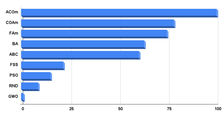
Fig. 4. Histogram of the final results of testing algorithms

Conclusions on the properties of the Bat Algorithm (BA):

Pros:
1. High speed.
2. The algorithm works well with smooth functions.
3. Scalability.

Cons:
1. Too many settings.
2. Mediocre results on discrete functions.