Population optimization algorithms: Evolution Strategies, (μ,λ)-ES and (μ+λ)-ES

Contents

1. Introduction
2. Algorithm
3. Replacing the test function
4. Test results
5. Conclusions

1. Introduction

Evolution Strategies algorithms are optimization methods based on principles observed in nature. They simulate natural selection, where the best solutions survive and pass on their characteristics to the next generation. These algorithms are widely used in solving optimization problems, especially in the fields of machine learning and artificial intelligence. They were developed in the 1960s by Professor Ingo Rechenberg and his colleagues in Germany to solve optimization problems in industry and engineering.

The basic idea of evolutionary strategies is to create a population of solutions and then improve them using mutation and selection operators similar to those used in natural evolution. Evolutionary strategies use real vectors to represent solutions. This allows us to more flexibly and accurately describe the solution space and search for optimal values in contrast to the classical genetic algorithm, which operates binary strings.

There are several different variants of evolutionary strategies, which differ in the way the population is generated and processed, as well as the mutation and selection operators used. Some of the most common options include:

1. (1+1)-ES: In this variant, only one child is created for each parent, and the best solution of the two becomes the parent for the next generation. This simple and fast method can be efficient for some problems, but is less effective when optimizing complex problems. The (1+1)-ES algorithm was created in the 1960s and is one of the simplest methods for optimization through evolutionary strategies. It consists of generating a random vector, which is then changed to a random step. If the modified vector is better, it replaces the original one, otherwise the original vector remains unchanged. This process is repeated until the optimum is achieved.

1. (μ,λ)-ES: In this algorithm, a population of μ size parents is created that produce λ children, and the best children replace the parents. It can be efficient for various optimization problems. The (μ,λ)-ES algorithm was created by Reinhard Speigelmann in 1965. After evaluating the children, only the best μ solutions are retained and become parents for the next generation, so parents are completely replaced by children at each epoch.

1. (μ+λ)-ES: In this option, λ descendants are created. The best of them, participate in the creation of the next generation together with their parents. In this method, parents and children compete with each other, which is an important difference from (μ,λ)-ES. The (μ+λ)-ES algorithm was created in the 1970s by Johannes Reichenbacher and Hans-Paul Schwefel and is a method for optimization through evolutionary strategies. This method allows for a more complete exploration of the solution space and can be more efficient in solving complex problems.

There are other variants of evolutionary strategies, but in this article we will consider only (μ,λ)-ES and (μ+λ)-ES. The (1+1)-ES option is simple and not suitable for solving multidimensional problems. Due to the difficulties in using the letters of the Greek alphabet and special characters in file names and variable names in the code, we will use PO and P_O, respectively, where P stands for parents and O means offspring (descendants).

Evolutionary strategies in computer science allow us to model evolution and natural selection to solve complex optimization problems. They use principles similar to natural selection to search for optimal solutions in parameter space.

These algorithms can be especially useful in problems where there is no obvious analytical solution or where the search space is very large. They can efficiently search for optimal solutions using evolution-inspired operations such as crossing, mutation and selection.

The name "Evolutionary Strategies" may be misleading, as researchers might think it is a general name for a class of evolutionary algorithms. However, this is not the case. In fact, it is a specific group of algorithms that use ideas of evolution to solve optimization problems.

2. Algorithm

(μ,λ)-ES means that at each iteration of the algorithm, μ parents are selected and λ children are generated. Then the best μ are selected from the λ children becoming the parents for the next iteration. Thus, in (μ,λ)-ES, new offspring completely replace their parents and participate in the creation of the next generation.

(μ+λ)-ES works in a similar way, but instead of selecting the best offspring from λ, they are combined with the parents to form a new population of μ+λ size. The best μ individuals are then selected from this combined population to become parents for the next iteration. Thus, in (μ+λ)-ES, new offspring work together with their parents to form the next population and compete with each other.

The main difference between (μ,λ)-ES and (μ+λ)-ES is how new offspring compete with parents for a place in the next population. In (μ,λ)-ES, new children compete with their parents for a limited number of places, which can lead to premature convergence to a local optimum. In (μ+λ)-ES, new children work together with their parents, resulting in a broader exploration of the solution space.

Both evolutionary strategy algorithms are based on a combination of genetic operators: mutation and selection. At each iteration of the algorithm, an individual is selected from the current population and the mutation operator is applied to it, after which the fitness of the resulting individual is calculated, and the fittest one is placed in the next population. To generate the initial population, an interval is specified for each component of the vector of varied parameters, and the initial values of the components are assumed to be uniformly distributed in the specified interval. The algorithm can use various stopping conditions, such as reaching a specified number of generations, a specified population state, or a specified level of convergence. In case of the (μ+λ) algorithm, all individuals are included in the population, while in case of the (μ,λ) algorithm, only descendants are included. For the (μ+λ) algorithm, convergence in probability has been proven, but for the (μ,λ) algorithm, the question of convergence remains open.

A comparison of the (μ+λ) and (μ,λ) algorithms shows that the (μ+λ) algorithm is more saving in using highly adapted individuals, leaving them to compete with descendants. This increases the intensity of the search, but can lead to premature convergence to a local extremum. The mutation operator in the canonical evolutionary strategy algorithm is the only evolutionary operator and uses the Gaussian mutation algorithm.

The classic (μ,λ)-ES algorithm can be described by the following pseudocode:

1. Initialize the initial population with random individuals.
2. Repeat until stopping criterion is reached:
2.1. Each of the μ parents generates λ offspring into the current population using the mutation operator.
2.2. Select the best μ descendants to form the next population.
3. Return the best individual from the last population.

The conventional (μ+λ)-ES algorithm can be described by the following pseudocode:

1. Initialize the initial population with random individuals.
2. Repeat until stopping criterion is reached:
2.1. Each of the μ parents generates λ offspring into the current population using the mutation operator.
2.2. Combine parents and offspring to obtain a combined population of μ+λ size.
2.3. Select the best μ individuals from the combined population to form the next one.
3. Return the best individual from the last population.

We looked at the classic versions of the two main "Evolutionary Strategies" algorithms. In both cases, parents produce λ offspring using only their genetic information. This results in star-shaped branching, where each descendant develops independently of the others. There is also no exchange of information between parents, which excludes the possibility of combining their genetic properties. As a result, combinatorial qualities are completely absent.

Test results showed that both of these ES options have low efficiency. I attempted to use recombination to increase it.

Recombination allows genetic material from different individuals to be combined to create new combinations that may have better properties or traits. This process promotes diversity in the population.

Recombination (or crossing) is the process of combining the genetic material of parents to create an offspring. This process simulates natural crossing in biological evolution. During recombination, the parents' genes combine to create new genetic material for the offspring. Recombination usually occurs at the level of genes or genetic traits. Genes are pieces of information in the genome that code for specific properties or characteristics of an organism.

After recombination, the genes of the descendant will be changed using the mutation operator, which makes random changes to the genes. This helps introduce new research variants into the population and promotes diversity in the genetic material.

Therefore, for each descendant gene we will use the genes of randomly selected parents, where gene is the corresponding coordinate of the parent. Thus, the offspring will inherit the characteristics of all parents in the population.

(μ,λ)-ES algorithm.

Let's move on to reviewing the code and start with a simpler algorithm (μ,λ)-ES modified by adding recombination (inheritance of genes from multiple parents).

For a parent and child acting as an agent, a good structure is S_Agent, which contains an array of coordinates "c" and a variable "f" - the fitness value. The Init function initializes the agent by resizing the array "c" and setting the value of "f" to "-DBL_MAX" (the worst possible fitness value).

//——————————————————————————————————————————————————————————————————————————————
struct S_Agent
{
  void Init (int coords)
  {
    ArrayResize (c, coords);
    f = -DBL_MAX;
  }

  double c []; //coordinates
  double f;    //fitness
};
//——————————————————————————————————————————————————————————————————————————————

Declare the C_AO_POES class to describe the (μ,λ)-ES algorithm.

The class contains the following elements:

• The "cB", "fB", "a", "rangeMax", "rangeMin", "rangeStep" public variables: These variables are used to store the best coordinate, corresponding fitness function value, agents, maximum and minimum search values and search step respectively.
• Public Init(): This function initializes the optimization algorithm. It takes several arguments such as the number of coordinates, population size, number of parent agents, mutation strength and sigma value. Inside the function, the variables and arrays used in the algorithm are initialized.
• "Moving()" and "Revision()" public functions: These functions are used to perform agent movement and population revision respectively.
• The "coords", "popSize", "parentsNumb", "mutationPower", "sigmaM" and "revision" private variables: These variables are used to store the number of coordinates, population size, number of parent agents, mutation strength, sigma value and revision flag respectively.
• The "parents", "ind", "val" and "pTemp" private arrays: These arrays are used to store information about parent agents, indices, values and temporary variables respectively.
• The GaussDistribution(), SeInDiSp(), RNDfromCI(), Scale(), Sorting() private functions: These functions are used to perform random number generation, value scaling and array sorting.

//——————————————————————————————————————————————————————————————————————————————
class C_AO_POES
{
  //----------------------------------------------------------------------------
  public: double  cB [];  //best coordinates
  public: double  fB;     //FF of the best coordinates
  public: S_Agent a  [];  //agent

  public: double rangeMax  []; //maximum search range
  public: double rangeMin  []; //manimum search range
  public: double rangeStep []; //step search

  public: void Init (const int    coordsP,          //coordinates number
                     const int    popSizeP,         //population size
                     const int    parentsP,         //number of parents, < Population size
                     const double mutationPowerP,   //mutation power
                     const double sigmaP);          //sigma

  public: void Moving   ();
  public: void Revision ();

  //----------------------------------------------------------------------------
  private: int    coords;        //coordinates number
  private: int    popSize;       //population size
  private: int    parentsNumb;   //number of parents
  private: double mutationPower; //mutation power
  private: double sigmaM;
  private: bool   revision;

  private: S_Agent parents [];  //parents
  private: int     ind     [];
  private: double  val     [];
  private: S_Agent pTemp   [];

  private: double GaussDistribution   (const double In, const double outMin, const double outMax, const double sigma);
  private: double SeInDiSp  (double In, double InMin, double InMax, double Step);
  private: double RNDfromCI (double min, double max);
  private: double Scale     (double In, double InMIN, double InMAX, double OutMIN, double OutMAX,  bool revers);
  private: void   Sorting   (S_Agent &p [], int size);
};
//——————————————————————————————————————————————————————————————————————————————

To initialize the optimization algorithm, use the Init function of the C_AO_POES class. The function takes several arguments: number of coordinates, population size, number of parent agents, mutation strength and sigma value.

Inside the function, the variables and arrays used in the algorithm are initialized. The function does the following:

• resets the random number generator and sets the "fB" variable to "-DBL_MAX". 
• sets the "coords", "popSize", "parentsNumb", "mutationPower" and "sigmaM" variable values. 
• changes the "ind", "val", "pTemp", "a", "parents", "rangeMax", "rangeMin", "rangeStep" and "cB" array size using the ArrayResize function. 
• the "a" and "parents" arrays are initialized using the Init function of the "S_Agent" class, which initializes the agent's coordinates and sets the value of the "f" variable to "-DBL_MAX".

//——————————————————————————————————————————————————————————————————————————————
void C_AO_POES::Init (const int    coordsP,          //coordinates number
                      const int    popSizeP,         //population size
                      const int    parentsP,         //number of parents, < Population size
                      const double mutationPowerP,   //mutation power
                      const double sigmaP)           //sigma
{
  MathSrand ((int)GetMicrosecondCount ()); // reset of the generator
  fB       = -DBL_MAX;
  revision = false;

  coords        = coordsP;
  popSize       = popSizeP;
  parentsNumb   = parentsP;
  mutationPower = mutationPowerP;
  sigmaM        = sigmaP;

  ArrayResize (ind,   popSize);
  ArrayResize (val,   popSize);
  ArrayResize (pTemp, popSize);
  ArrayResize (a,     popSize);
  for (int i = 0; i < popSize; i++) a [i].Init (coords);

  ArrayResize (parents, parentsNumb);
  for (int i = 0; i < parentsNumb; i++) parents [i].Init (coords);

  ArrayResize (rangeMax,  coords);
  ArrayResize (rangeMin,  coords);
  ArrayResize (rangeStep, coords);
  ArrayResize (cB,        coords);
}
//——————————————————————————————————————————————————————————————————————————————

The Moving method moves agents in the search space.

The function contains two blocks of code separated by the "if (!revision)" condition.

1. In the first block, random coordinates are generated for each agent if the "revision" flag is "false". For each coordinate, a random number is generated with a uniform distribution between "rangeMin" and "rangeMax", then this number is normalized using the SeInDiSp function, which sets the coordinate value to the nearest multiple of "rangeStep".
2. In the second block, the movement of agents occurs if the "revision" flag is equal to "true". For each agent, a random parent agent is selected from the "parents" array. Then, the mutation value "dist" is calculated for each agent coordinate. The value depends on the "mutationPower" mutation strength and the "rangeMin" and "rangeMax" search range. The agent's coordinate value is changed using the GaussDistribution function, which generates a normally distributed random number around the parent coordinate value using the "sigmaM" sigma value. The coordinate value is then normalized using the SeInDiSp function.
   

//——————————————————————————————————————————————————————————————————————————————
void C_AO_POES::Moving ()
{
  //----------------------------------------------------------------------------
  if (!revision)
  {
    for (int i = 0; i < popSize; i++)
    {
      for (int c = 0; c < coords; c++)
      {
        a [i].c [c] = RNDfromCI (rangeMin [c], rangeMax [c]);
        a [i].c [c] = SeInDiSp (a [i].c [c], rangeMin [c], rangeMax [c], rangeStep [c]);
      }
    }

    revision = true;
    return;
  }

  //----------------------------------------------------------------------------
  int    indx = 0;
  double min  = 0.0;
  double max  = 0.0;
  double dist = 0.0;

  for (int i = 0; i < popSize; i++)
  {
    for (int c = 0; c < coords; c++)
    {
      indx = (int)RNDfromCI (0, parentsNumb);
      if (indx >= parentsNumb) indx = parentsNumb - 1;

      a [i].c [c] = parents [indx].c [c];

      dist = (rangeMax [c] - rangeMin [c]) * mutationPower;

      min = a [i].c [c] - dist; if (min < rangeMin [c]) min = rangeMin [c];
      max = a [i].c [c] + dist; if (max > rangeMax [c]) max = rangeMax [c];

      a [i].c [c] = GaussDistribution (a [i].c [c], min, max, sigmaM);
      a [i].c [c] = SeInDiSp  (a [i].c [c], rangeMin [c], rangeMax [c], rangeStep [c]);
    }
  }
}
//——————————————————————————————————————————————————————————————————————————————

The population revision is performed by the "Revision" method, which is used to revise the current state of agents in the optimization algorithm.

The function contains two blocks of code.

1. In the first block, the best agent is searched for in the "a" array using the "for" loop. If an agent is found with a higher fitness value than the current best agent "fB", then the index of that agent is stored in the "indx" variable. The "fB" value and "cB" coordinates of the current best agent are then updated according to the new best agent.
2. In the second block, the "a" array is sorted in descending order of fitness using the Sorting function, and then the "parentsNumb" of the best agents from the "a" array is copied to the "parents" array.

Thus, the "Revision" function allows updating the current state of agents and save the best agents in the "parents" array, where the best children completely replace all parents.

//——————————————————————————————————————————————————————————————————————————————
void C_AO_POES::Revision ()
{
  //----------------------------------------------------------------------------
  int indx = -1;

  for (int i = 0; i < popSize; i++)
  {
    if (a [i].f > fB) indx = i;
  }

  if (indx != -1)
  {
    fB = a [indx].f;
    ArrayCopy (cB, a [indx].c, 0, 0, WHOLE_ARRAY);
  }

  //----------------------------------------------------------------------------
  Sorting (a, popSize);
  for (int i = 0; i < parentsNumb; i++)
  {
    parents [i] = a [i];
  }
}
//——————————————————————————————————————————————————————————————————————————————

(μ+λ)-ES algorithm.

Changes begin with adding the life expectancy of an individual in the form of the "yearsNumber" parameter. This makes it possible to control the maximum age in the population and avoid "clogging" it with very old individuals, which can prevent the exploration of new horizons of infinite living space and making new discoveries. I hope, this will be useful in this algorithm.

Why is this counter not included in the "(μ,λ)-ES" algorithm? Because that is how it was intended. Parents are completely replaced with descendants. This also makes sense, as is the case with semeloges in the animal kingdom, where some species reproduce only once in their lives. Examples of such species include salmonids, agaves, bamboo, coconut crabs and cycads. However, in our algorithm we will give the opportunity for individuals to reproduce several times, live indefinitely or die like a proud bamboo. Life expectancy can be an adjustable external parameter, and as part of our testing, the optimal duration of 10 years was experimentally found.

In addition, a life counter can help avoid "overfitting" the model, when the population begins to "remember" and accumulate specific solutions rather than finding new successful solutions elsewhere in the search space. Limiting the lifespan of individuals allows us to maintain the diversity of the population and continue to look for more optimal solutions.

//——————————————————————————————————————————————————————————————————————————————
struct S_Agent
{
  void Init (int coords)
  {
    ArrayResize (c, coords);
    f = -DBL_MAX;
    yearsNumber = 0;
  }

  double c []; //coordinates
  double f;    //fitness
  int yearsNumber;
};
//——————————————————————————————————————————————————————————————————————————————

In the "Init" method, we will increase the size of the parent population by the number of children. This will allow parents and children to be sorted together, although, as in the (μ,λ)-ES algorithm, in the future only the μ part of the joint population will be used to generate new children. While in the previous algorithm, the number of parents had to be less than or equal to the population of descendants, then in this algorithm it does not matter and the population of parents can be set to any size, even very large. This does not affect the number of epochs. It was experimentally found that the parent population of 150 is the optimal value in case of 100 offspring (a greater value is not possible as the number of epochs decreases). A further increase in the population of parents leads to too much diversity in the gene pool and the algorithm begins to converge worse (this is interesting in itself).

ArrayResize (ind,   popSize + parentsNumb);
ArrayResize (val,   popSize + parentsNumb);
ArrayResize (pTemp, popSize + parentsNumb);
ArrayResize (a,     popSize);
for (int i = 0; i < popSize; i++) a [i].Init (coords);

ArrayResize (parents, popSize + parentsNumb);
for (int i = 0; i < popSize + parentsNumb; i++) parents [i].Init (coords);

In the Moving method, set the individual's year counter to 1 when creating new descendants.

a [i].yearsNumber = 1;

The changes also affected the Revision method, in which the code performs the following taking into account the changes:

• Increase the value of "yearsNumber" of each parent by 1.
• If the value of "yearsNumber" exceeds the specified limit (lifespan), it sets the fitness value "f" for the corresponding parent to "-DBL_MAX", which means removing the individual from the population.
  
• Copies the new children from the "a" array to the "parents" array.
• Sorts the "parents" array by the "f" fitness value.

//----------------------------------------------------------------------------
for (int i = 0; i < parentsNumb; i++)
{
  parents [i].yearsNumber++;

  if (parents [i].yearsNumber > lifespan)
  {
    parents [i].f = - DBL_MAX;
  }
}

for (int i = parentsNumb; i < parentsNumb + popSize; i++)
{
  parents [i] = a [i - parentsNumb];
}

Sorting (parents, parentsNumb + popSize);

3. Replacing the test function

Previously, we used the Rastrigin function as a test function to evaluate optimization algorithms. However, the Rastrigin function is not a perfect choice for such purposes. It has strict periodicity and balanced minimums and maximums, which can be detected relatively easily by some algorithms. Thus, the Rastrigin function exhibits patterns that may affect the algorithm's ability to determine the extrema of the function.

For more reliable and objective testing of optimization algorithms, it is recommended to use functions with diverse and unpredictable properties. Such functions usually do not have obvious patterns or balance between minimums and maximums. Examples of such functions include noise functions, functions with non-linear dependencies or functions with a large number of local extrema. This choice of functions allows us to more accurately assess the ability of algorithms to detect and converge to global optima under various conditions.

Conventionally, all functions can be divided into "simple" and "complex". Simple functions are those whose most surface area lies above the midline between 'max' and 'min', and the more surface area lies closer to 'max', the simpler it is for optimization algorithms. So, if we simply randomly place points over the entire surface in the domain of the function, we will get a false impression of "high" optimization results, since the results will be close to the absolute global maximum. An example of such a simple function is the schematic drawing of the hypothetical function in Fig. 1.

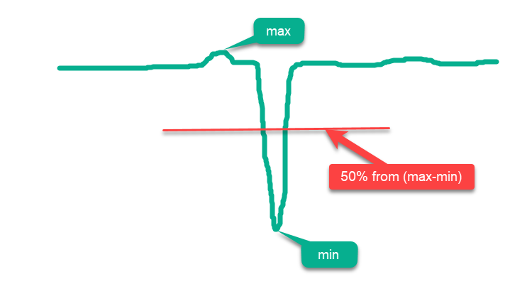
Figure 1. An example of a "simple" function for optimization algorithms

In view of the above, the Rastrigin function can be classified as a simple function that may cause inflated results for some optimization algorithms. This is due to the peculiarities of the search strategy of these algorithms, which can place their agents dispersed across the entire function surface.

The impact is especially noticeable on Rastrigin functions with a large number of variables, for example 1000. While some algorithms "honestly" try to find the global extremum, others may simply place agents evenly across the entire surface of the function. This approach does not indicate the ability of the optimization algorithm to perform an accurate search, but only gives the illusion of being able to do so.

The Rastrigin function has been significantly modified to create a more complex and challenging environment for optimization algorithms. The new version of the function has added several "hills" and "valleys", while maintaining periodicity in that part of the surface that does not help in finding the global extremum. These changes create additional obstacles, distracting agents and acting as traps.

Now we cannot just jump on steps that have a periodicity to reach a global extreme, as was the case in the conventional version of Rastrigin. In addition, the global optimum has been shifted away from the edge, making it difficult to find in case of artifacts in the algorithms that often focus on the boundaries of the function definition.

The new function is called "Hilly" (Fig. 2). Like "Forest" and "Megacity", it refers to complex test functions. For these three functions, the surface area lying above 50% of the maximum height is approximately the same and constitutes about 20% of the total area of the function.

The Hilly, Forest and Megacity functions provide complex and realistic optimization scenarios that can help evaluate the performance of algorithms under complex and varied conditions. By using these functions as a comprehensive test of optimization algorithms, we can gain more insight into their ability to find global optima and overcome local pitfalls.

In addition, changes have been made to the testing methodology. Now 10-fold testing is carried out instead of 5-fold (the number of repeated runs of the optimization process) to reduce random "spikes" in the results.

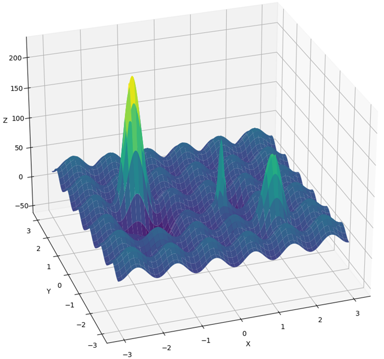
Figure 2. Hilly test function

4. Test results

(μ,λ)-ES algorithm test stand results:

C_AO_(PO)ES:100:10:0.025:8.0
=============================
5 Hilly's; Func runs: 10000; result: 0.7902459324049909
25 Hilly's; Func runs: 10000; result: 0.6264667539839893
500 Hilly's; Func runs: 10000; result: 0.42934981087827656
=============================
5 Forest's; Func runs: 10000; result: 0.8761631782479373
25 Forest's; Func runs: 10000; result: 0.6094343681829253
500 Forest's; Func runs: 10000; result: 0.19591138782930953
=============================
5 Megacity's; Func runs: 10000; result: 0.5900000000000001
25 Megacity's; Func runs: 10000; result: 0.37933333333333336
500 Megacity's; Func runs: 10000; result: 0.11321666666666666
=============================
All score: 4.61012

(μ+λ)-ES algorithm test stand results:

C_AO_(P_O)ES:100:150:0.02:8.0:10
=============================
5 Hilly's; Func runs: 10000; result: 0.9993447297882565
25 Hilly's; Func runs: 10000; result: 0.9189524317647721
500 Hilly's; Func runs: 10000; result: 0.562968579605404
=============================
5 Forest's; Func runs: 10000; result: 1.0
25 Forest's; Func runs: 10000; result: 0.9352215748931851
500 Forest's; Func runs: 10000; result: 0.3917923122543615
=============================
5 Megacity's; Func runs: 10000; result: 0.8316666666666664
25 Megacity's; Func runs: 10000; result: 0.6443333333333332
500 Megacity's; Func runs: 10000; result: 0.21155000000000007
=============================
All score: 6.49583

The visualization below is for the (μ+λ)-ES algorithm, which demonstrates excellent exploration of the search space without leaving out potentially promising areas.

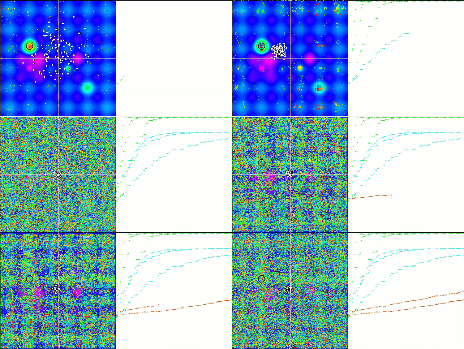
(μ+λ)-ES on the Hilly test function

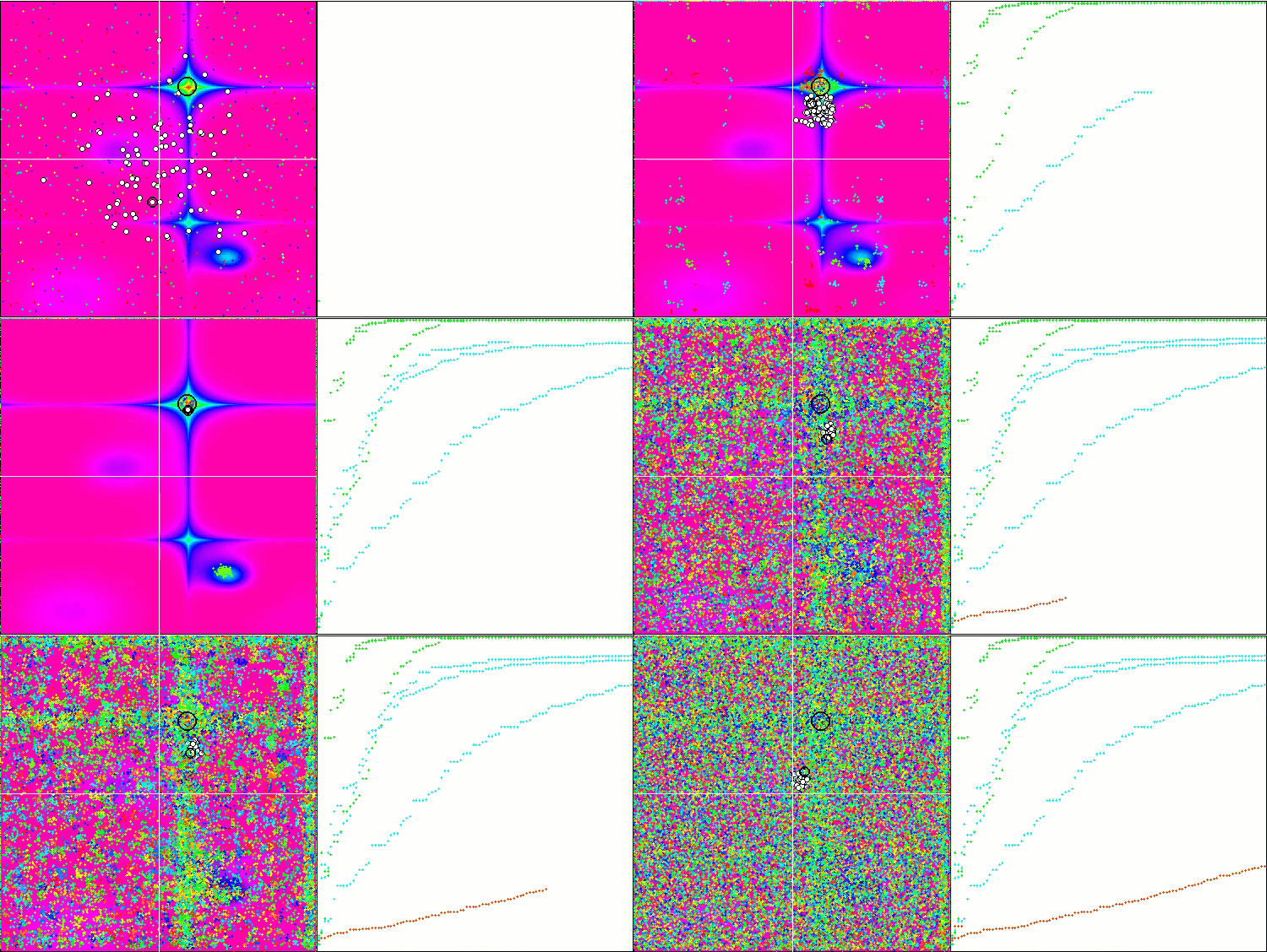
  (μ+λ)-ES on the Forest test function

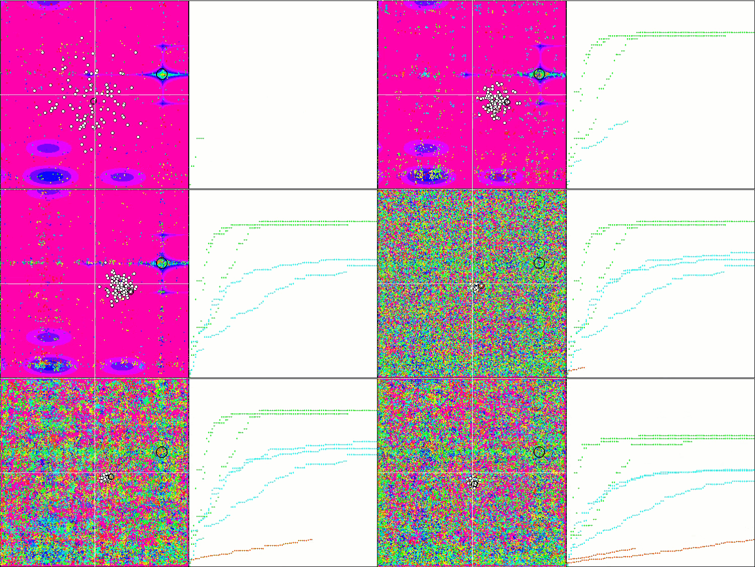
  (μ+λ)-ES on the Megacity test function

It was decided to return to absolute values of test results and abandon relative ones. To achieve this, the test functions were modified so that they returned values in the range from 0.0 to 1.0. Now, if the result is 1.0, it means 100% convergence, while 0.32527 means 32.5% of the global maximum of the test function. Thus, since the total number of tests is 9, theoretically the algorithms can show the maximum possible total result for all tests of no more than 9.0 in the case of 100% convergence of the algorithm on each test in the "Final result" column of the table. Additionally, the "% of MAX" column has been added showing the percentage of the maximum possible result.

Now the result numbers will not change when new algorithms are added to the table since they are presented in absolute values.

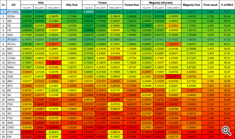
So, let's move on to the results of the considered algorithms, first of all (μ+λ)-ES. This algorithm really amazed me with its phenomenal results: it scored a total of 72.18% of the theoretically possible result. To ensure these impressive results, 20-fold testing was carried out specifically for this algorithm. Each of the 20 runs showed 100% convergence on the complex Forest function - this is simply enormous! In addition, the results on other functions were also remarkable.

Now some good words about (μ,λ)-ES. This algorithm demonstrated stable and good results. In the color graph, it is uniformly "green" with no sudden color changes.

#	AO	Description	Hilly			Hilly final	Forest			Forest final	Megacity (discrete)			Megacity final	Final result	% of MAX
			10 p (5 F)	50 p (25 F)	1000 p (500 F)		10 p (5 F)	50 p (25 F)	1000 p (500 F)		10 p (5 F)	50 p (25 F)	1000 p (500 F)
1	(P+O)ES	(P+O) evolution strategies	0.99934	0.91895	0.56297	2.48127	1.00000	0.93522	0.39179	2.32701	0.83167	0.64433	0.21155	1.68755	6.496	72.18
2	SDSm	stochastic diffusion search M	0.93066	0.85445	0.39476	2.17988	0.99983	0.89244	0.19619	2.08846	0.72333	0.61100	0.10670	1.44103	5.709	63.44
3	SIA	simulated isotropic annealing	0.95784	0.84264	0.41465	2.21513	0.98239	0.79586	0.20507	1.98332	0.68667	0.49300	0.09053	1.27020	5.469	60.76
4	DE	differential evolution	0.95044	0.61674	0.30308	1.87026	0.95317	0.78896	0.16652	1.90865	0.78667	0.36033	0.02953	1.17653	4.955	55.06
5	HS	harmony search	0.86509	0.68782	0.32527	1.87818	0.99999	0.68002	0.09590	1.77592	0.62000	0.42267	0.05458	1.09725	4.751	52.79
6	SSG	saplings sowing and growing	0.77839	0.64925	0.39543	1.82308	0.85973	0.62467	0.17429	1.65869	0.64667	0.44133	0.10598	1.19398	4.676	51.95
7	(PO)ES	(PO) evolution strategies	0.79025	0.62647	0.42935	1.84606	0.87616	0.60943	0.19591	1.68151	0.59000	0.37933	0.11322	1.08255	4.610	51.22
8	ACOm	ant colony optimization M	0.88190	0.66127	0.30377	1.84693	0.85873	0.58680	0.15051	1.59604	0.59667	0.37333	0.02472	0.99472	4.438	49.31
9	MEC	mind evolutionary computation	0.69533	0.53376	0.32661	1.55569	0.72464	0.33036	0.07198	1.12698	0.52500	0.22000	0.04198	0.78698	3.470	38.55
10	IWO	invasive weed optimization	0.72679	0.52256	0.33123	1.58058	0.70756	0.33955	0.07484	1.12196	0.42333	0.23067	0.04617	0.70017	3.403	37.81
11	COAm	cuckoo optimization algorithm M	0.75820	0.48652	0.31369	1.55841	0.74054	0.28051	0.05599	1.07704	0.50500	0.17467	0.03380	0.71347	3.349	37.21
12	SDOm	spiral dynamics optimization M	0.74601	0.44623	0.29687	1.48912	0.70204	0.34678	0.10944	1.15826	0.42833	0.16767	0.03663	0.63263	3.280	36.44
13	NMm	Nelder-Mead method M	0.73807	0.50598	0.31342	1.55747	0.63674	0.28302	0.08221	1.00197	0.44667	0.18667	0.04028	0.67362	3.233	35.92
14	FAm	firefly algorithm M	0.58634	0.47228	0.32276	1.38138	0.68467	0.37439	0.10908	1.16814	0.28667	0.16467	0.04722	0.49855	3.048	33.87
15	GSA	gravitational search algorithm	0.64757	0.49197	0.30062	1.44016	0.53962	0.36353	0.09945	1.00260	0.32667	0.12200	0.01917	0.46783	2.911	32.34
16	ABC	artificial bee colony	0.63377	0.42402	0.30892	1.36671	0.55103	0.21874	0.05623	0.82600	0.34000	0.14200	0.03102	0.51302	2.706	30.06
17	BFO	bacterial foraging optimization	0.54626	0.43533	0.31907	1.30066	0.41626	0.23156	0.06266	0.71048	0.35500	0.15233	0.03627	0.54360	2.555	28.39
18	BA	bat algorithm	0.59761	0.45911	0.35242	1.40915	0.40321	0.19313	0.07175	0.66810	0.21000	0.10100	0.03517	0.34617	2.423	26.93
19	SA	simulated annealing	0.55787	0.42177	0.31549	1.29513	0.34998	0.15259	0.05023	0.55280	0.31167	0.10033	0.02883	0.44083	2.289	25.43
20	IWDm	intelligent water drops M	0.54501	0.37897	0.30124	1.22522	0.46104	0.14704	0.04369	0.65177	0.25833	0.09700	0.02308	0.37842	2.255	25.06
21	PSO	particle swarm optimisation	0.59726	0.36923	0.29928	1.26577	0.37237	0.16324	0.07010	0.60572	0.25667	0.08000	0.02157	0.35823	2.230	24.77
22	MA	monkey algorithm	0.59107	0.42681	0.31816	1.33604	0.31138	0.14069	0.06612	0.51819	0.22833	0.08567	0.02790	0.34190	2.196	24.40
23	SFL	shuffled frog-leaping	0.53925	0.35816	0.29809	1.19551	0.37141	0.11427	0.04051	0.52618	0.27167	0.08667	0.02402	0.38235	2.104	23.38
24	FSS	fish school search	0.55669	0.39992	0.31172	1.26833	0.31009	0.11889	0.04569	0.47467	0.21167	0.07633	0.02488	0.31288	2.056	22.84
25	RND	random	0.52033	0.36068	0.30133	1.18234	0.31335	0.11787	0.04354	0.47476	0.25333	0.07933	0.02382	0.35648	2.014	22.37
26	GWO	grey wolf optimizer	0.59169	0.36561	0.29595	1.25326	0.24499	0.09047	0.03612	0.37158	0.27667	0.08567	0.02170	0.38403	2.009	22.32
27	CSS	charged system search	0.44252	0.35454	0.35201	1.14907	0.24140	0.11345	0.06814	0.42299	0.18333	0.06300	0.02322	0.26955	1.842	20.46
28	EM	electroMagnetism-like algorithm	0.46250	0.34594	0.32285	1.13129	0.21245	0.09783	0.10057	0.41085	0.15667	0.06033	0.02712	0.24412	1.786	19.85

Figure 3. Color gradation of algorithms according to relevant tests

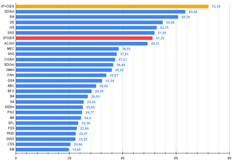
Figure 4. The histogram of algorithm test results (on a scale from 0 to 100, the more the better,

where 100 is the maximum possible theoretical result (the archive features a script for calculating the rating table).

5. Summary

The use of evolutionary strategies opens up new possibilities in various fields, including parameter optimization in machine learning, robot design and control of complex systems. They allow us to obtain better solutions based on the biological principles of evolution.

We have a new undisputed leader in the table at the moment, which is ahead of its nearest competitor SDSm by almost 10%.

(μ,λ)-ES algorithm pros and cons:

Advantages:

1. Small number of external parameters.
2. High efficiency in solving a variety of problems.
3. Ease of implementation.
4. Resistance to sticking.
5. Promising results on both smooth and complex discrete functions.
6. High convergence.

Disadvantages:

1. Large scatter of results on discrete functions.
   

(μ+λ)-ES algorithm pros and cons:

Advantages:

1. Small number of external parameters.
2. High efficiency in solving a variety of problems.
3. Ease of implementation.
4. Resistance to sticking.
5. Promising results on both smooth and complex discrete functions.
6. High convergence.

Disadvantages:

1. Large scatter of results on discrete functions (although these are the best results at the moment).

The article is accompanied by an archive with updated current versions of the algorithm codes described in previous articles. The author of the article is not responsible for the absolute accuracy in the description of canonical algorithms. Changes have been made to many of them to improve search capabilities. The conclusions and judgments presented in the articles are based on the results of the experiments.