Econometrics: bibliography
The following references are available on the subject of "Fundamentals of Regression Analysis".
Davidson,Russell and James G. MacKinnon (1993). Estimation and Inference inEconometrics, Oxford: Oxford University Press.
Greene, William H. (2008). Econometric Analysis, 6th Edition, Upper Saddle River, NJ: Prentice-Hall.
Johnston, Jack and John Enrico DiNardo (1997). Econometric Methods, 4th Edition, New York: McGraw-Hill.
Pindyck, Robert S. and Daniel L. Rubinfeld (1998). Econometric Models and Economic Forecasts, 4th edition, New York: McGraw-Hill.
Wooldridge, Jeffrey M. (2000). Introductory Econometrics: A Modern Approach. Cincinnati, OH: South-Western College Publishing.
Let me give you an example of a regression, which is nothing but a function (dependent variable) that depends on its arguments (independent variables, regressors). There are several steps to follow when calculating a regression:
1. An equation needs to be written down.
I take the hotly favoured MA, but weighted, so forgiving for me, calculating it using the previous 5 bars (lag values). I write the formula in the form:
EURUSD = C(1)*EURUSD(-1) + C(2)*EURUSD(-2) + C(3)*EURUSD(-3) + C(4)*EURUSD(-4) + C(5)*EURUSD(-5)
2. estimate
It is necessary to estimate the coefficient c(i) of this equation so that the curve of our MA corresponds to the initial EURUSD_H1-year series as good as possible. We obtain the result of the evaluation of the unknown coefficients.
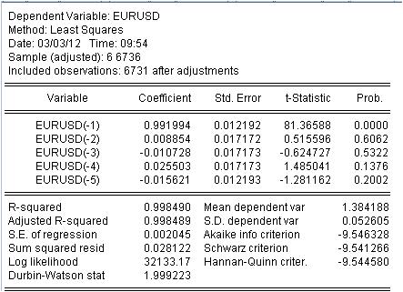
We have obtained the values of our weighted MA. We have the equation:
EURUSD = 0.991993934254*EURUSD(-1) + 0.00885362355538*EURUSD(-2) - 0.0107282369642*EURUSD(-3) + 0.0255027160774*EURUSD(-4) - 0.0156205779585*EURUSD(-5)
3. Results.
What results do we see?
3.1 First of all the Mach equation itself. I want to pay attention to a little nuance. When we calculate a simple mask calculating the average, we do not record it in the middle of the interval but at its end for some reason. The regression is used to calculate the latest value based on the previous ones.
3.2 It turns out, that ratios are not constants, but random variables with their own deviation.
3.3. The last column says that there is a non-zero probability that the coefficients given are zero at all.
4. Working with the equation
Let's take a look at our weighted mixture.

The mashka has covered the cotier so tightly that it cannot be seen, but there are still discrepancies between the cotier and the mashka. Here are the statistics of these discrepancies

We see a huge scatter from -137 points to 215 points. Though standard deviation = 20 points.
Conclusion.
We have received an unusually high quality of the mask with the known statistical characteristics using regression.
The last one. Yusuf! Don't get under the tram, don't make the audience laugh on one more thread.
Ready to discuss the literature and application of the regression topic.
3. Results.
What results do we see?
3.1 First of all, the Mach equation itself. I want to point out one subtlety here. When we calculate a simple mask by getting the average, for some reason we do not place this average in the middle of the interval, but at its end. The regression is used to calculate the latest value based on the previous ones.
3.2 It turns out, that ratios are not constants, but random variables!
3.3 The last column says that there is a non-zero probability that the given coefficients are zero.
1. sorry for the extra salt in the wound - the original series is non-stationary anyway.
2) This probability is almost always non-zero.
3. have you checked for multicollinearity? IMHO if you eliminate multicollinearity there is only one variable left. Have you determined the significant factors?
4. How many observations do you have for 5 variables?
How are you so literate?
1. sorry for the extra salt in the wound - the original series is non-stationary anyway.
Of course, we are not interested in the others.
2. That probability is almost always non-zero.
Not true. If non-zero, it's a functional form error.
3. have you checked for multicollinearity? IMHO if you eliminate multicollinearity there is only one variable left. Have you identified the significant factors?
What are "significant factors" I do not understand, but please look at correlation coefficients.
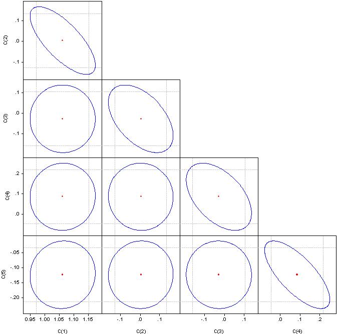
If it's a circle, the correlation is zero. If merged into a straight line, the correlation between the corresponding pair of coefficients is 100%.
4. How many observations do you have for 5 variables?
6736 observations
The first step in any regression model is factor selection. If you don't apply stepwise regression (with inclusions or exclusions), then you have to select them manually.
Multicollinearity - close dependence between factor variables included in the model. Not the correlation of the coefficients, but the correlation of the factors.
The presence of multicollinearity leads to:
- distortion of the value of the parameters of the model, which tend to overestimate;
- weak conditioning of the system of normal equations;
- complication of the process of determining the most significant factor features.
One indicator of multicollinearity is that pairwise correlation coefficients exceed the value of 0.8. Here the factors clearly have a strong correlation. In order to eliminate it we need to remove redundant factors. Either manually or by stepwise regression.
Look in the package - step regression or ridge regression.
And 6736/4 is too many observations. We need to google - I don't remember how to determine the optimal number of observations based on the number of factors.
Be so kind as to participate in my econometrics threads.
Let's continue with the literature selection.
Next topic is Almon's lags.
As noted above, there are difficulties with regression coefficients calculated using the method of least squares. An idea has emerged to impose additional constraints on the regression coefficients in which the dependent variable is determined by several lags of the independent variable as in the equation above.
The idea is to impose constraints on the coefficients at lag values such that they obey some polynomial distribution. EViews calls this approach "distributed lag polynomials (PDL)". The choice of the particular degree of polynomial is determined experimentally.
This approach is described here.
Here is a practical example.
Let's construct an analogue of a scale with a period of 5, but the bar coefficients should be on a polynomial of 3rd order.
In EViews it is written as follows for EURUSD
EURUSD PDL(EURUSD(-1), 5,3)
In a more familiar form:
EURUSD = + C(5)*EURUSD(-1) + C(6)*EURUSD(-2) + C(7)*EURUSD(-3) + C(8)*EURUSD(-4) + C(9)*EURUSD(-5) + C(10)*EURUSD(-6)
We estimate the coefficients by OLS and get the result of the coefficient estimation:
EURUSD = + 0.934972661616*EURUSD(-1) + 0.139869148138*EURUSD(-2) - 0.093599954464*EURUSD(-3) - 0.0264992987207*EURUSD(-4) + 0.0801064628352*EURUSD(-5) - 0.0348473223286*EURUSD(-6)
The statistics on the estimation of the equation is as follows:
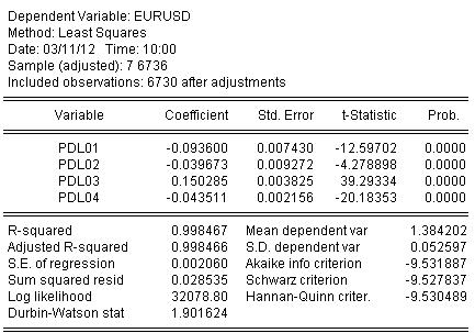
From the statistics we can see a very good level of mapping of the initial quotient by our waving from Almon R-square = 0.998467
Graphically it looks like:

The regression (Almon's waving) has completely covered the original quotient.
And one last spoon of honey.
Let's see what the residual is, i.e. the difference between our Almon's mash and the original cotier. The stationarity/non-stationarity of this residual is very important.
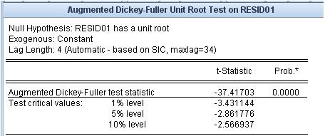
The unit root test states that the residual is stationary.
The mash-ups we use do not have this level of fit to the original quotient and the stationarity property of the fitting error.
I would like to move the links from a neighbouring thread.
These links relate to the most problematic area - prognosis.
The first one is an attachment. there is a list of references.
- Free trading apps
- Over 8,000 signals for copying
- Economic news for exploring financial markets
You agree to website policy and terms of use
If you Google the word "econometrics", you will get a huge list of literature, which is difficult to understand even for an expert. One book says one thing, another - another, the third - just a compilation of the first two with some inaccuracies. But the "from the books" approach combines not clarity of application of these books in practice. I'm not interested in intellectuals descending into nerdish nonsense.
Similarly to other lists of books in this forum, for example, on statistics, I propose that we collectively compile a list of textbooks, monographs, dissertations, articles, Internet resources and software packages which, in the opinion of participants, would be relevant to the measurement of economic data - to econometrics. However, let us not forget that mathematical statistics is the older sister of econometrics. I suggest not including anything related to technical analysis in this list.
To exclude sliding into botany, I propose a specific approach to the list of books. We post links (books themselves) only if I know software, which implements algorithms from these books. I have narrowed it down to EViews. This program has no advantage over others, it has advantages and disadvantages, but I take it as a rubricator for econometrics. I have attached the table of contents of the second volume of the user's manual, in order to outline at once the widest possible range of problems. Due to the proposed approach, several areas used in econometrics, but not included in EVIEWS, e.g. NS, wavelets, etc., are excluded. Naturally references to such programs and books are also welcome.
If we can not only provide a link to the source of the algorithm, but also make specific calculations, this thread will be of no value.
I suggest using chapter numbers from the attachment for book grouping.
So, please support.