
Building Your First Glass-box Model Using Python And MQL5
Introduction
Glass-box algorithms are machine learning algorithms that are fully transparent and inherently intelligible. They defy conventional wisdom that there is a tradeoff between prediction accuracy and interpretability in Machine Learning because they offer an unparalleled level of accuracy and transparency. This means they are exponentially easier to debug, maintain, and improve upon iteration when compared to their black-box alternatives that we are more familiar with. Black-box models are all machine learning models whose inner workings are complex and not easily interpretable. These models can represent high dimensional and non-linear relationships which aren't easily understood by us as humans.
As a rule of thumb, black-box models should only be used in scenarios where a glass-box model cannot deliver the same level of accuracy. In this article we will build a glass-box model and understand the potential benefits of employing them. We will explore 2 ways of controlling our MetaTrader 5 terminal with our glass-box model:
- Legacy Approach: This is the easiest approach possible. We simply connect our glass-box model to our MetaTrader 5 Terminal using the integrated Python library in MetaTrader 5. From there we will build an Expert Advisor in MetaQuotes Language 5 to assist our glass-box model and maximize our effectiveness.
- Contemporary Approach: This is the recommended way of integrating Machine Learning models into your expert advisor. We will export our glass-box model to Open Neural Network Exchange format and then load the model directly into our Expert Advisor as a resource allowing us to leverage all the useful features available in MetaTrader 5 and fuse it with the power of our glass-box model.

Figure 1: Mimicking The Human Brain Using Artificial Intelligence
Black-box Models Vs Glass-box Models
As aforementioned, most traditional machine learning models are difficult to interpret or explain. This class of models is known as black-box models. Black-box models encompass all models with complex and non-easily interpretable inner workings. This poses a major problem for us as we try improving our model's key performance metrics. Glass-box models, on the other hand, are a set of machine learning models whose inner workings are transparent and intelligible and furthermore their prediction accuracy is also high and reliable.
Researchers, Developers, and an ensemble of Domain Experts at Microsoft Research open sourced and at the time of writing actively maintain a Python package called Interpret ML. The package contains a comprehensive suite of black-box explainers and glass-box models. Black-box explainers are a set of algorithms that try to gain insight into the inner workings of a black-box model. Most of the black-box explainer algorithms in Interpret ML are model agnostic, meaning they can be applied on any black-box model. However, these black-box explainers can only give estimations of the black-box models, we will explore why this can be problematic in the next section of this article. Interpret ML also includes a suite of glass-box models, these models rival the prediction accuracy of black-box models with unprecedented transparency. This is perfect for anyone using Machine Learning whether a beginner or an expert, the value of model interpretability transcends domain and experience level.
For additional information:
1. If you are interested, you can read the Interpret ML documentation.
2. Furthermore you can read through the Interpret ML white paper.
We will use Interpret ML in this paper to build a glass-box model in python. We will see how our glass-box model can give us crucial insight to guide our feature engineering process and improve our understanding of our model's inner workings.
The Challenge of Black-box Models: The Disagreement Problem
One of the reasons we might want to stop using black-box models is referred to as the "Disagreement Problem". In a nutshell, different explanation techniques can give very different model explanations even if they are assessing the same model. Explanation techniques attempt to gain insight into the underlying structure of a black-box model. There are many different schools of thought encompassing model explanations, and because of that each explanation technique may focus on different aspects of model behavior and therefore they can each infer different metrics about the underlying black-box model. The Disagreement problem is an open area of research and is a caveat to be recognized and proactively mitigated.
In this paper we will observe a real-life demonstration of the disagreement problem in case the reader has not observed this phenomenon independently.
For additional information:
1. If you are interested in learning more about the disagreement problem, I recommend reading this excellent research paper from a bright collective of Harvard, MIT, Drexel and Carnegie Mellon university alumni.
Without further ado let's see the disagreement problem in action:
First, we import python packages to help us perform our analysis.
#Import MetaTrader5 Python package
#pip install --upgrade MetaTrader5, if you don't have it installed
import MetaTrader5 as mt5

#Import datetime for selecting data
#Standard python package, no installation required
from datetime import datetime

#Plotting Data
#pip install --upgrade matplotlib, if you don't have it installed
import matplotlib.pyplot as plt

#Import pandas for handling data
#pip install --upgrade pandas, if you don't have it installed
import pandas as pd

#Import library for calculating technical indicators
#pip install --upgrade pandas-ta, if you don't have it installed
import pandas_ta as ta

#Scoring metric to assess model accuracy
#pip install --upgrade scikit-learn, if you don't have it installed
from sklearn.metrics import precision_score

#Import mutual information, a black-box explanation technique
from sklearn.feature_selection import mutual_info_classif

#Import permutation importance, another black-box explanation technique
from sklearn.inspection import permutation_importance

#Import our model
#pip install --upgrade xgboost, if you don't have it installed
from xgboost import XGBClassifier

#Plotting model importance
from xgboost import plot_importance
From there we can move on to connecting to our MetaTrader 5 terminal, but before that we have to specify our login credentials.
#Enter your account number
login = 123456789

#Enter your password
password = '_enter_your_password_'

#Enter your Broker's server
server = 'Deriv-Demo'
Now we can initialize the MetaTrader 5 Terminal and login to our trading account in the same step.
#We can initialize the MT5 terminal and login to our account in the same step
if mt5.initialize(login=login,password=password,server=server):
    print('Logged in successfully')
else:
    print('Failed To Log in')
Logged in successfully.
We now have full access the MetaTrader 5 terminal and request chart data, tick data, current quotes and much more.
#To view all available symbols from your broker
symbols = mt5.symbols_get()

for index,value in enumerate(symbols):
    print(value.name)
Volatility 10 Index
Volatility 25 Index
Volatility 50 Index
Volatility 75 Index
Volatility 100 Index
Volatility 10 (1s) Index
Boom 1000 Index
Boom 500 Index
Crash 1000 Index
Crash 500 Index
Step Index
...
Once we've identified which symbol we want to model, we can request chart data on that symbol, but first we need to specify the range of dates we want to pull.
#We need to specify the dates we want to use in our dataset
date_from = datetime(2019,4,17)
date_to = datetime.now()
Now we can request chart data on that symbol.
#Fetching historical data
data = pd.DataFrame(mt5.copy_rates_range('Boom 1000 Index',mt5.TIMEFRAME_D1,date_from,date_to))
We need to format the time column in our dataframe for plotting purposes.
#Let's convert the time from seconds to year-month-date
data['time'] = pd.to_datetime(data['time'],unit='s')

data
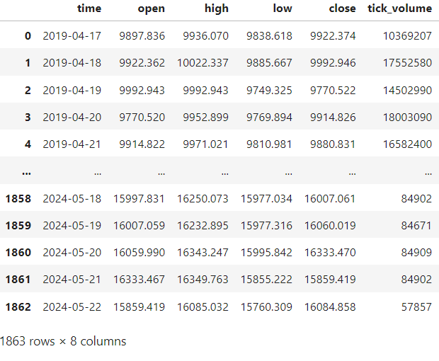
Fig 2: Our DataFrame now displays time in human readable format. Notice that the "real_volume" column is filled with zeros.
Now we need to create a helper function to help us add new features to our dataframe, calculate technical indicators and clean up our dataframe.
#Let's create a function to preprocess our data
def preprocess(df):
    #All values of real_volume are 0 in this dataset, we can drop the column
    df.drop(columns={'real_volume'},inplace=True)
    #Calculating 14 period ATR
    df.ta.atr(length=14,append=True)
    #Calculating the growth in the value of the ATR, the second difference
    df['ATR Growth'] = df['ATRr_14'].diff().diff()
    #Calculating 14 period RSI
    df.ta.rsi(length=14,append=True)
    #Calculating the rolling standard deviation of the RSI
    df['RSI Stdv'] = df['RSI_14'].rolling(window=14).std()
    #Calculating the mid point of the high and low price
    df['mid_point'] = ( ( df['high'] + df['low'] ) / 2 )
    #We will keep track of the midpoint value of the previous day
    df['mid_point - 1'] = df['mid_point'].shift(1)
    #How far is our price from the midpoint?
    df['height'] = df['close'] - df['mid_point']
    #Drop any rows that have missing values
    df.dropna(axis=0,inplace=True)
Let's call the preprocess function on our dataframe.
preprocess(data)

data
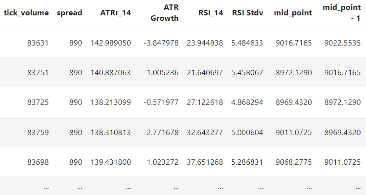
Fig 3: Our dataframe has now been preprocessed.
Our target will be whether the next close price is greater than today's close price. We will use dummy encoding for this, if tomorrow's close price is greater than today's close price our target will be 1. Otherwise, our target will be 0.
#We want to predict whether tomorrow's close will be greater than today's close
#We can encode a dummy variable for that:
#1 means tomorrow's close will be greater.
#0 means today's close will be greater than tomorrow's.

data['target'] = (data['close'].shift(-1) > data['close']).astype(int)

data

#The first date is 2019-05-14, and the first close price is 9029.486, the close on the next day 2019-05-15 was 8944.461
#So therefore, on the first day, 2019-05-14, the correct forecast is 0 because the close price fell the following day.
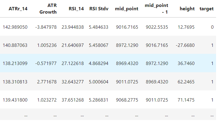
Fig 4: Creating our target
Next, we explicitly define our target and our predictors. Then we split our data into training and testing sets. Note that this is timeseries data therefore we cannot randomly split into 2 groups.
#Seperating predictors and target
predictors = ['open','high','low','close','tick_volume','spread','ATRr_14','ATR Growth','RSI_14','RSI Stdv','mid_point','mid_point - 1','height']
target     = ['target']

#The training and testing split definition
train_start = 27
train_end = 1000

test_start = 1001
Now we create the training and testing sets.
#Train set
train_x = data.loc[train_start:train_end,predictors]
train_y = data.loc[train_start:train_end,target]

#Test set
test_x = data.loc[test_start:,predictors]
test_y = data.loc[test_start:,target]
Now we can fit our black-box model.
#Let us fit our model
black_box = XGBClassifier()
black_box.fit(train_x,train_y)
Let's see our model's predictions on the test set.
#Let's see our model predictions
black_box_predictions = pd.DataFrame(black_box.predict(test_x),index=test_x.index)
Let's assess our model's accuracy.
#Assesing model prediction accuracy
black_box_score = precision_score(test_y,black_box_predictions)

#Model precision score
black_box_score
0.4594594594594595
Our model is 45% accurate, which features are helping us achieve this and which ones aren't? Fortunately, XGBoost comes packaged with an inbuilt function to measure feature importance making our lives easier. However, this is specific to this implementation of XGBoost, and not all black-boxes contain useful functions to easily show feature importance in such a manner. For example, neural networks and support vector machines don't have an equivalent function, you'd have to soberly analyze and carefully interpret the model weights by yourself to understand your model better. The plot_importance function in XGBoost allows us to peek inside our model.
plot_importance(black_box)
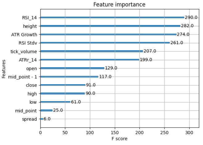
Fig 5: The feature importance of our XGBClassifier. Notice that the table doesn't include any interaction terms, does that mean none exist? Not necessarily!
Now that we've established the ground truth, let's look at our first black-box explanation technique called "Permutation importance". Permutation importance attempts to estimate the importance of each feature by randomly shuffling the values in each feature and then measuring the change in the model's loss function. The reasoning is that the more your model relies on that feature the worse its performance will be if we randomly shuffle those values. Let's discuss some of the advantages and disadvantages of Permutation Importance
Advantages
- Model agnostic: Permutation importance can be used on any black-box model without any preprocessing needed to either the model or the permutation importance function, this makes it easy to integrate into your existing machine learning workflow.
- Interpretability: The results of permutation importance are easy to interpret and are interpreted consistently regardless of the underlying model being assessed. This makes it a straightforward tool to use.
- Handles non-linearity: Permutation importance is robust and is suitable for capturing non-linear relationships between the predictors and the response.
- Handles outliers: Permutation importance doesn't rely on the raw values of the predictors; it is concerned with the impact of the features on the model's performance. This approach makes it robust to outliers that may be in the raw data.
Disadvantages
- Computational cost: For large datasets with many features, calculating permutation importance can be computationally expensive, because we must iterate over each feature, permute it and assess the model, then move on to the next feature and repeat the process.
- Challenged by correlated features: Permutation importance may give biased results when assessing features that are strongly correlated.
- Sensitive to model complexity: Though permutation importance is model agnostic it is possible that an overly complex model will exhibit high variance when its features are permuted, making it challenging to draw reliable conclusions.
- Feature independence: Permutation importance assumes that features in the dataset are independent and can be permuted randomly without consequence. This makes calculations easier but in the real world most features are dependent on each other and have interactions that will not be picked up by permutation importance.
Let's calculate permutation importance for our black-box classifier.
#Now let us observe the disagreement problem
black_box_pi = permutation_importance(black_box,train_x,train_y)

# Get feature importances and standard deviations
perm_importances = black_box_pi.importances_mean
perm_std = black_box_pi.importances_std

# Sort features based on importance
sorted_idx = perm_importances.argsort()
Let's plot our calculated permutation importance values.
#We're going to utilize a bar histogram
plt.barh(range(train_x.shape[1]), perm_importances[sorted_idx], xerr=perm_std[sorted_idx])
plt.yticks(range(train_x.shape[1]), train_x.columns[sorted_idx])
plt.xlabel('Permutation Importance')
plt.title('Permutation Importances')
plt.show() 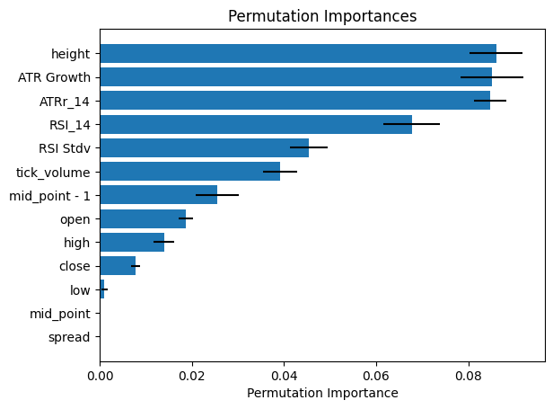
Fig 6: Permutation Importance for our black-box
According to the calculations performed by the permutation importance algorithm, the ATR reading is the most informative feature we have engineered. But we know from our ground truth that it's not, the ATR ranked sixth. The ATR growth is the most important feature! The second most important feature was the height, however permutation importance calculated that the ATR Growth was more important. The third most important feature was the RSI reading but our permutation importance calculated height as being more important.
This is the problem with black-box explanation techniques, they are very good estimates of feature importance however they are prone to be wrong because at best they are only estimations. And not only that, but they can also disagree with each other when evaluating the same model. Let's see this for ourselves.
We will use the mutual information algorithm as our second black-box explanation technique. Mutual information measures the reduction in uncertainty that is brought about by being aware of a feature's value.
#Let's see if our black-box explainers will disagree with each other by calculating mutual information
black_box_mi = mutual_info_classif(train_x,train_y)
black_box_mi = pd.Series(black_box_mi, name="MI Scores", index=train_x.columns)
black_box_mi = black_box_mi.sort_values(ascending=False)

black_box_mi
RSI_14: 0.014579
open: 0.010044
low: 0.005544
mid_point - 1: 0.005514
close: 0.002428
tick_volume : 0.001402
high: 0.000000
spread: 0.000000
ATRr_14: 0.000000
ATR Growth: 0.000000
RSI Stdv: 0.000000
mid_point: 0.000000
height: 0.000000
Name: MI Scores, dtype: float64
As you can see, we have wildly different importance rankings. Mutual information is ranking the features in almost reverse order compared to our ground truth and the permutation importance calculation. If you didn't have the ground truth that we have in this example, which explainer were you going to rely on more? Furthermore, what if you used 5 different explanation techniques and they each gave you different importance rankings, then what? Do you pick the rankings that align with your beliefs about the workings of the real world, that opens the door to another problem called confirmation bias. Confirmation bias is when you disregard any evidence that contradicts your existing beliefs, you actively seek to validate what you believe is the truth even if it's not true!
The Advantages of Glass-box Models
Glass-box models perfectly substitute the need for black-box explanation techniques because they are fully transparent and very intelligible. They hold the potential to solve the disagreement problem across many domains, including our financial domain. If that wasn't reason enough, debugging a glass-box model is exponentially easier than debugging a black-box model of the same level of flexibility. This saves our most important resource of all, time! And the best part is that it doesn't compromise model accuracy by being a glass-box, giving us the best of both worlds. As a rule of thumb black-boxes should only be used in scenarios where a glass-box cannot achieve the same level off accuracy.
With that out of the way let us now turn our attention to building our first glass-box model, analyzing its performance, and trying to improve its accuracy. From there we will cover how to connect our glass-box model to our MetaTrader 5 Terminal and start trading with glass-box models. Then we will build an Expert Advisor that will assist our glass-box model using MetaQuotes Language 5. And lastly, we will export our glass-box model to Open Neural Network Exchange Format so that we can unleash the full potential of MetaTrader 5 and our glass-box model.
Building Your First Glass-box Model Using Python Is Easy
To keep the code easy to read, we will build our glass-box in a separate python script from the python script we used to build the black-box model, however most things will remain the same, such as logging in, fetching data, and preprocessing the data. Therefore, we won't go over those steps again, we'll only focus on the steps unique to the glass-box model.
To get started we first need to install Interpret ML
#Installing Interpret ML
pip install --upgrade interpret
Then we load our dependencies. In this article we will focus on 3 modules in the interpret package. The first one is the glass-box model itself, and the second is a useful module that allows us to look inside the model and presents this information in an interactive GUI dashboard and the last package allows us to visualize our model's performance in one graph. The other packages have already been discussed.
#Import MetaTrader5 package
import MetaTrader5 as mt5

#Import datetime for selecting data
from datetime import datetime

#Import matplotlib for plotting
import matplotlib.pyplot as plt

#Intepret glass-box model for classification
from interpret.glassbox import ExplainableBoostingClassifier

#Intepret GUI dashboard utility
from interpret import show

#Visualising our model's performance in one graph
from interpret.perf import ROC

#Pandas for handling data
import pandas as pd

#Pandas-ta for calculating technical indicators
import pandas_ta as ta

#Scoring metric to assess model accuracy
from sklearn.metrics import precision_score
We then create our login credentials and login to our MT5 terminal as we did before. This step is omitted.
From there select the symbol you want to model as we did before. This step is omitted.
Then we specify the date range for the data we want to model as we did before. This step is omitted.
Then we can fetch the historical data as we did before. This step is omitted.
From there we follow the same preprocessing steps as outlined above. This step is omitted.
Once the data has been preprocessed, we then add our target as did before. This step is omitted.
We then perform our train test split as we did before. This step is omitted. Make sure that your train test split is not randomized. Preserve the natural time order otherwise your results will be compromised and paint an overly optimistic picture of future performance.
Now we fit our glass-box model.
#Let us fit our glass-box model
#Please note this step can take a while, depending on your computational resources
glass_box = ExplainableBoostingClassifier()
glass_box.fit(train_x,train_y)
We can now look inside our glass-box model
#The show function provides an interactive GUI dashboard for us to interface with out model
#The explain_global() function helps us find what our model found important and allows us to identify potential bias or unintended flaws
show(glass_box.explain_global())
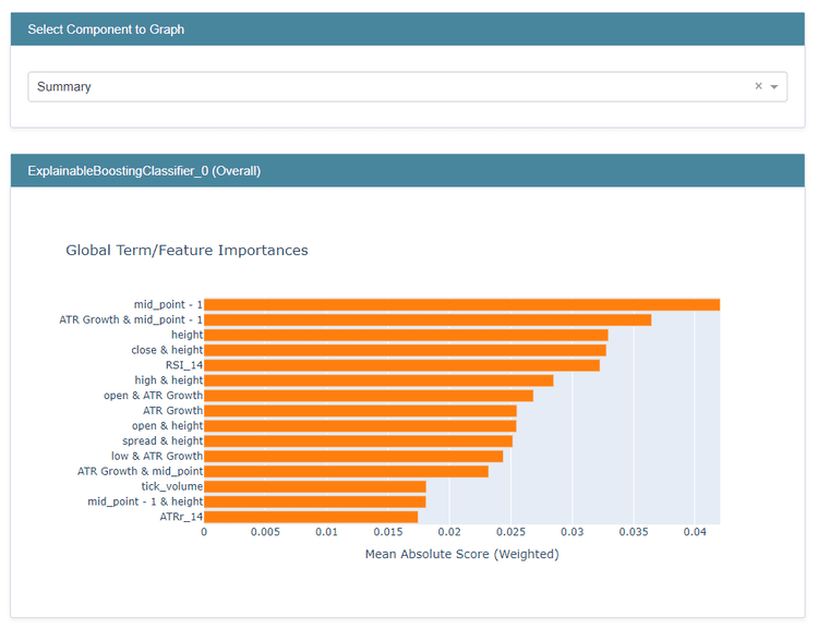
Fig 7: Glass-box Global State
Interpreting the summary statistics is very important. But before we go there let's first go over some important nomenclature. "Global Term" or "Global State" summarizes the entire model's state. It gives us an overview of which features the model found informative. This is not to be confused with "Local Term" or "Local State". Local states are used to explain individual model predictions to help us understand why the model made the prediction it made and which features influenced individual predictions.
Back to the global state of our glass-box model. As we can see the model found the lagged midpoint value very informative which is what we expected. Not only that but it also found a possible interaction term between the ATR Growth and the lagged midpoint value. The height was the third most important feature followed by an interaction term between the close price and the height. Note that we don't need any additional tools whatsoever to understand our glass-box model, this completely shuts the door on the disagreement problem and confirmation bias. The Global State information is invaluable in terms of feature engineering because it shows us where we could direct our future efforts for engineering better features. Moving on, let's see how our glass-box performs.
Obtaining glass-box predictions
#Obtaining glass-box predictions
glass_box_predictions = pd.DataFrame(glass_box.predict(test_x))
Now we measure the glass-box accuracy.
glass_box_score = precision_score(test_y,glass_box_predictions)

glass_box_score
0.49095022624434387
Our glass-box has an accuracy of 49%. Clearly our Explainable Boosting Classifier can pull its own weight when compared to our XGBClassifier. This just goes to demonstrate the power of glass-box models to give us high accuracy without compromising intelligibility.
We can also obtain individual explanations for each prediction from our glass-box model, to understand which features influenced its prediction at a granular level, these are called Local Explanations and obtaining them from our Explainable Boosting Classifier is straight forward
#We can also obtain individual explanations for each prediction
show(glass_box.explain_local(test_x,test_y))
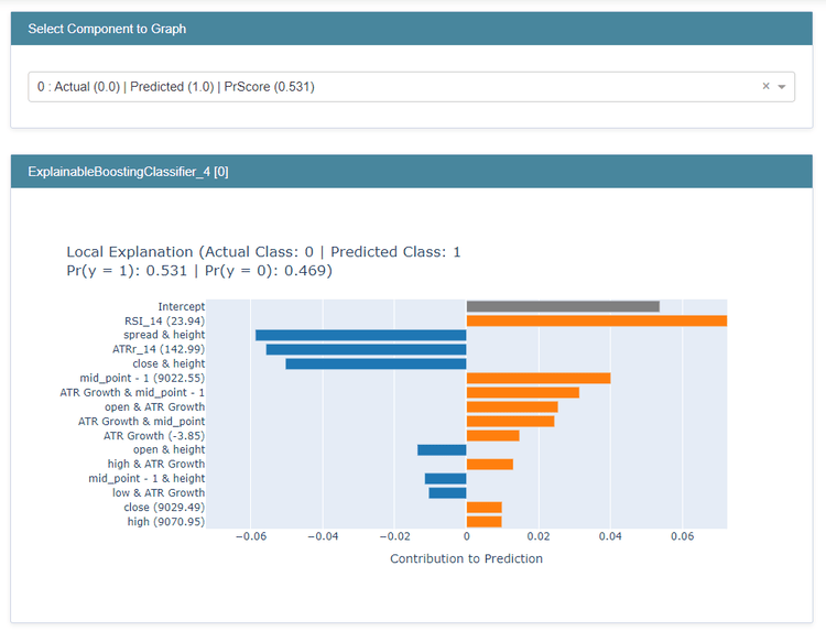
Fig 8: Local explanations from our Explainable Boosting Classifier
The first drop down menu allows us to scroll through each of the predictions made and select the prediction we want to understand better.
From there we can see the actual class vs the predicted class. In this case the actual class was 0, meaning the close price fell, but we classified it as 1. We are also presented with the estimated probabilities of each class respectively, as we can see our model incorrectly estimated a 53% probability that the next candle would close higher. We are also given a breakdown of the contribution made by each feature to the estimated probability. The features in blue we're contributing against the prediction made by our model, and the features in orange were responsible for the prediction made by our model. So that means the RSI contributed the most to this misclassification but the interaction term between the spread and the height was pointing us in the right direction, these features may be worth engineering further but a more rigorous examination of the local explanations is needed before we can reach any conclusions.
We will now examine our model's performance with a single graph known as the Receiver Operating Characteristic or ROC. The ROC graph allows us to assess the performance of our classifier in a simple manner. We are concerned with the area under the curve or the AUC. In theory a perfect classifier will have a total area under the curve of 1. This makes it easy to assess our classifier with just one graph.
glass_box_performance = ROC(glass_box.predict_proba).explain_perf(test_x,test_y, name='Glass Box')
show(glass_box_performance)
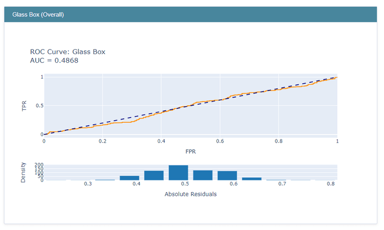
Fig 9: The ROC chart of our glass-box model
Our glass-box model has an AUC of 0.49. This simple metric lets us assess our model's performance using units that are interpretable to us as humans, and furthermore the curve is model agnostic and can be used to compare different classifiers regardless of the underlying classification techniques.
Connecting Your Glass-box Model To Your MT5 Terminal
This is where the rubber meets the road, we will now connect our glass-box model to our MT5 terminal using the simpler approach first.
First let's track our current account standing.
#Fetching account Info
account_info = mt5.account_info()

# getting specific account data
initial_balance = account_info.balance
initial_equity = account_info.equity

print('balance: ', initial_balance)
print('equity: ', initial_equity)
balance: 912.11 equity: 912.11
Fetch all symbols.
symbols = mt5.symbols_get()
Let's set up some global variables.
#Trading global variables
#The symbol we want to trade
MARKET_SYMBOL = 'Boom 1000 Index'

#This data frame will store the most recent price update
last_close = pd.DataFrame()

#We may not always enter at the price we want, how much deviation can we tolerate?
DEVIATION = 100

#For demonstrational purposes we will always enter at the minimum volume
#However,we will not hardcode the minimum volume, we will fetch it dynamically
VOLUME = 0
#How many times the minimum volume should our positions be
LOT_MUTLIPLE = 1

#What timeframe are we working on?
TIMEFRAME = mt5.TIMEFRAME_D1
We don't want to hardcode the trading volume; we'd rather get the minimum allowed trading volume dynamically from broker and then multiply it by some factor to ensure that we don't send invalid orders. So, in this paper we'll think of our order sizes relative to the minimum volume.
In our case we will open every trade at minimum volume or using a factor of 1.
for index,symbol in enumerate(symbols):
    if symbol.name == MARKET_SYMBOL:
        print(f"{symbol.name} has minimum volume: {symbol.volume_min}")
        VOLUME = symbol.volume_min * LOT_MULTIPLE
Boom 1000 Index has minimum volume: 0.2
Now we'll define a helper function to open trades.
# function to send a market order
def market_order(symbol, volume, order_type, **kwargs):
    #Fetching the current bid and ask prices
    tick = mt5.symbol_info_tick(symbol)

    #Creating a dictionary to keep track of order direction
    order_dict = {'buy': 0, 'sell': 1}
    price_dict = {'buy': tick.ask, 'sell': tick.bid}

    request = {
        "action": mt5.TRADE_ACTION_DEAL,
        "symbol": symbol,
        "volume": volume,
        "type": order_dict[order_type],
        "price": price_dict[order_type],
        "deviation": DEVIATION,
        "magic": 100,
        "comment": "Glass Box Market Order",
        "type_time": mt5.ORDER_TIME_GTC,
        "type_filling": mt5.ORDER_FILLING_FOK,
    }

    order_result = mt5.order_send(request)
    print(order_result)
    return order_result
Next, we'll define a helper function to close trades based on ticket number.
# Closing our order based on ticket id
def close_order(ticket):
    positions = mt5.positions_get()

    for pos in positions:
        tick = mt5.symbol_info_tick(pos.symbol) #validating that the order is for this symbol
        type_dict = {0: 1, 1: 0}  # 0 represents buy, 1 represents sell - inverting order_type to close the position
        price_dict = {0: tick.ask, 1: tick.bid} #bid ask prices

        if pos.ticket == ticket:
            request = {
                "action": mt5.TRADE_ACTION_DEAL,
                "position": pos.ticket,
                "symbol": pos.symbol,
                "volume": pos.volume,
                "type": type_dict[pos.type],
                "price": price_dict[pos.type],
                "deviation": DEVIATION,
                "magic": 100,
                "comment": "Glass Box Close Order",
                "type_time": mt5.ORDER_TIME_GTC,
                "type_filling": mt5.ORDER_FILLING_FOK,
            }

            order_result = mt5.order_send(request)
            print(order_result)
            return order_result

    return 'Ticket does not exist'
We don't need to keep requesting a lot of data from the server, so we'll also update our date range.
#Update our date from and date to
date_from = datetime(2023,11,1)
date_to = datetime.now()
We also need a function to get a forecast from our glass-box model and use the forecast as trading signals.
#Get signals from our glass-box model
def ai_signal():
    #Fetch OHLC data
    df = pd.DataFrame(mt5.copy_rates_range(market_symbol,TIMEFRAME,date_from,date_to))
    #Process the data
    df['time'] = pd.to_datetime(df['time'],unit='s')
    df['target'] = (df['close'].shift(-1) > df['close']).astype(int)
    preprocess(df)
    #Select the last row
    last_close = df.iloc[-1:,1:]
    #Remove the target column
    last_close.pop('target')
    #Use the last row to generate a forecast from our glass-box model
    #Remember 1 means buy and 0 means sell
    forecast = glass_box.predict(last_close)
    return forecast[0]
Now we define the main body of our Python glass-box Trading Bot
#Now we define the main body of our Python Glass-box Trading Bot
if __name__ == '__main__':
    #We'll use an infinite loop to keep the program running
    while True:
        #Fetching model prediction
        signal = ai_signal()

        #Decoding model prediction into an action
        if signal == 1:
            direction = 'buy'
        elif signal == 0:
            direction = 'sell'

        print(f'AI Forecast: {direction}')

        #Opening A Buy Trade
        #But first we need to ensure there are no opposite trades open on the same symbol
        if direction == 'buy':
            #Close any sell positions
            for pos in mt5.positions_get():
                if pos.type == 1:
                    #This is an open sell order, and we need to close it
                    close_order(pos.ticket)

            if not mt5.positions_totoal():
                #We have no open positions
                market_order(MARKET_SYMBOL,VOLUME,direction)

        #Opening A Sell Trade
        elif direction == 'sell':
            #Close any buy positions
            for pos in mt5.positions_get():
                if pos.type == 0:
                    #This is an open buy order, and we need to close it
                    close_order(pos.ticket)

            if not mt5.positions_get():
                #We have no open positions
                market_order(MARKET_SYMBOL,VOLUME,direction)

        print('time: ', datetime.now())
        print('-------\n')
        time.sleep(60)
AI Forecast: sell
OrderSendResult(retcode=10009, deal=3830247156, order=3917630794, volume=0.2, price=16042.867, bid=16042.867, ask=16044.37, comment='Request executed', request_id=4013241765, retcode_external=0, request=TradeRequest(action=1, magic=100, order=0, symbol='Boom 1000 Index', volume=0.2, price=16042.883, stoplimit=0.0, sl=0.0, tp=0.0, deviation=100, type=1, type_filling=0, type_time=0, expiration=0, comment='Glass Box Market Order', position=0, position_by=0))
time: 2024-05-22 19:04:17.842750
-------
AI Forecast: sell
time: 2024-05-22 19:05:17.904601
-------
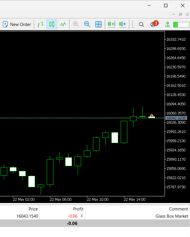
Fig 10: Our Glass-box Trading Bot Built In Python Is Profiting
Building An Expert Advisor to Assist Your Glass-box Model
We now move on to building an assistant for our glass-box model using MQL5. We want to build an EA that will move our stop-loss (SL) and take-profit (TP) based on an ATR reading. The code below will update our TP and SL values on every tick, performing this task using the Python integration module would be a nightmare unless you update at lower frequencies such as per minute or per hour. We want to run a tight ship and update our SL and TP on every tick, anything else won't satisfy our strict requirements. We will need two inputs from our user specifying how large the gap between the entry and the SL/TP should be. We will multiply the ATR reading by the user input to determine calculate the height from either the SL or TP to the point of entry. And the second input is simply the period of the ATR.
//Meta Properties
#property copyright "Gamuchirai Ndawana"
#property link "https://twitter.com/Westwood267"

//Classes for managing Trades And Orders
#include  <Trade\Trade.mqh>
#include <Trade\OrderInfo.mqh>

//Instatiating the trade class and order manager
CTrade trade;
class COrderInfo;

//Input variables
input double atr_multiple =0.025;  //How many times the ATR should the SL & TP be?
input int atr_period = 200;      //ATR Period

//Global variables
double ask, bid,atr_stop; //We will use these variables to determine where we should place our ATR
double atr_reading[];     //We will store our ATR readings in this arrays
int    atr;               //This will be our indicator handle for our ATR indicator
int min_volume;

int OnInit(){
                  //Check if we are authorized to use an EA on the terminal
                  if(!TerminalInfoInteger(TERMINAL_TRADE_ALLOWED)){
                           Comment("Press Ctrl + E To Give The Robot Permission To Trade And Reload The Program");
                           //Remove the EA from the terminal
                           ExpertRemove();
                           return(INIT_FAILED);
                  }

                  //Check if we are authorized to use an EA on the terminal
                  else if(!MQLInfoInteger(MQL_TRADE_ALLOWED)){
                            Comment("Reload The Program And Make Sure You Clicked Allow Algo Trading");
                            //Remove the EA from the terminal
                            ExpertRemove();
                            return(INIT_FAILED);
                  }

                  //If we arrive here then we are allowed to trade using an EA on the Terminal
                  else{
                        //Symbol information
                        //The smallest distance between our point of entry and the stop loss
                        min_volume = SymbolInfoInteger(_Symbol,SYMBOL_TRADE_STOPS_LEVEL);//SymbolInfoDouble(_Symbol,SYMBOL_VOLUME_MIN)
                        //Setting up our ATR indicator
                        atr = iATR(_Symbol,PERIOD_CURRENT,atr_period);
                        return(INIT_SUCCEEDED);
                  }
}

void OnDeinit(const int reason){

}

void OnTick(){
               //Get the current ask
               ask = SymbolInfoDouble(_Symbol,SYMBOL_ASK);
               //Get the current bid
               bid = SymbolInfoDouble(_Symbol,SYMBOL_BID);
               //Copy the ATR reading our array for storing the ATR value
               CopyBuffer(atr,0,0,1,atr_reading);
               //Set the array as series so the natural time ordering is preserved
               ArraySetAsSeries(atr_reading,true);

               //Calculating where to position our stop loss
               //For now we'll keep it simple, we'll add the minimum volume and the current ATR reading and multiply it by the ATR multiple
               atr_stop = ((min_volume + atr_reading[0]) * atr_multiple);

               //If we have open positions we should adjust the stop loss and take profit
               if(PositionsTotal() > 0){
                        check_atr_stop();
               }
}

//--- Functions
//This funciton will update our S/L & T/P based on our ATR reading
void check_atr_stop(){

      //First we iterate over the total number of open positions
      for(int i = PositionsTotal() -1; i >= 0; i--){

            //Then we fetch the name of the symbol of the open position
            string symbol = PositionGetSymbol(i);

            //Before going any furhter we need to ensure that the symbol of the position matches the symbol we're trading
                  if(_Symbol == symbol){
                           //Now we get information about the position
                           ulong ticket = PositionGetInteger(POSITION_TICKET); //Position Ticket
                           double position_price = PositionGetDouble(POSITION_PRICE_OPEN); //Position Open Price
                           double type = PositionGetInteger(POSITION_TYPE); //Position Type
                           double current_stop_loss = PositionGetDouble(POSITION_SL); //Current Stop loss value

                           //If the position is a buy
                           if(type == POSITION_TYPE_BUY){
                                  //The new stop loss value is just the ask price minus the ATR stop we calculated above
                                  double atr_stop_loss = (ask - (atr_stop));
                                  //The new take profit is just the ask price plus the ATR stop we calculated above
                                  double atr_take_profit = (ask + (atr_stop));

                                  //If our current stop loss is less than our calculated ATR stop loss
                                  //Or if our current stop loss is 0 then we will modify the stop loss and take profit
                                 if((current_stop_loss < atr_stop_loss) || (current_stop_loss == 0)){
                                       trade.PositionModify(ticket,atr_stop_loss,atr_take_profit);
                                 }
                           }

                            //If the position is a sell
                           else if(type == POSITION_TYPE_SELL){
                                     //The new stop loss value is just the bid price plus the ATR stop we calculated above
                                     double atr_stop_loss = (bid + (atr_stop));
                                     //The new take profit is just the bid price minus the ATR stop we calculated above
                                     double atr_take_profit = (bid - (atr_stop));

                                 //If our current stop loss is greater than our calculated ATR stop loss
                                 //Or if our current stop loss is 0 then we will modify the stop loss and take profit
                                 if((current_stop_loss > atr_stop_loss) || (current_stop_loss == 0)){
                                       trade.PositionModify(ticket,atr_stop_loss,atr_take_profit);
                                 }
                           }
                  }
            }
}
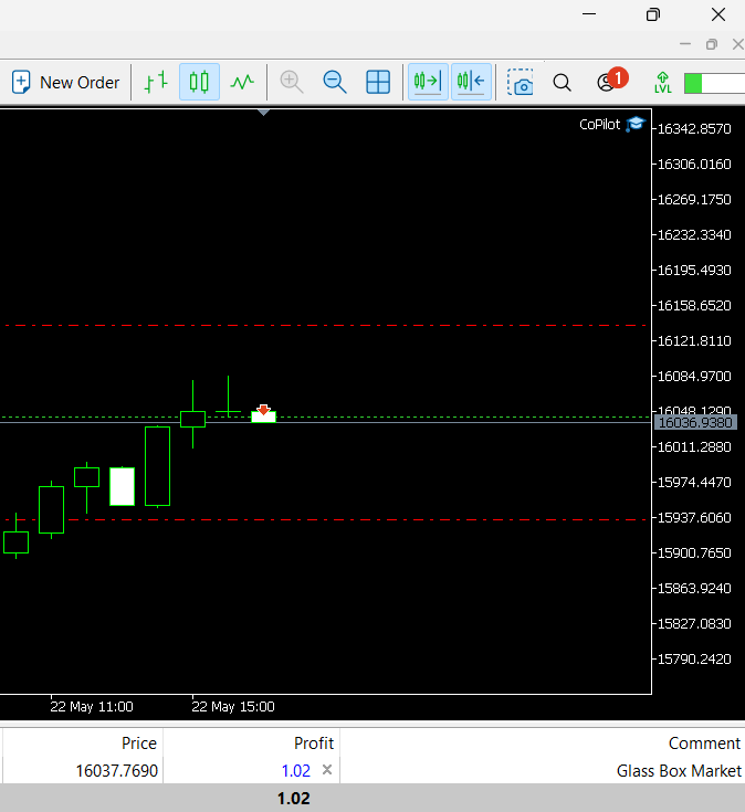
Fig 11: Our EA is working hand in hand with our Glass-box Model
Exporting Our Glass-box Model to Open Neural Network Exchange (ONNX) Format

Fig 12: The Open Neural Network Exchange Logo
Open Neural Network Exchange (ONNX) is an opensource protocol for representing any machine learning model. It is widely supported and maintained by a large widespread collective effort of companies from around the world and from different industries. Companies such as Microsoft, Facebook, MATLAB, IBM, Qualcomm, Huawei, Intel, AMD just to name a few. At the time of writing ONNX is the universal standard form for representing any machine learning model regardless of which framework it was developed in, and furthermore it allows machine learning models to be developed and deployed in different programming languages and environments. If you’re curious how this is possible, the core idea is that any machine learning model can be represented as a graph of nodes and edges. Each node represents a mathematical operation, and each edge represents the flow of data. Using this simple representation, we can represent any machine learning model regardless of the framework that made it.
Once you have an ONNX model you need to have the engine which runs ONNX models, this is the responsibility of the ONNX Runtime. The ONNX Runtime is responsible for efficiently running and deploying ONNX models on a variety of devices from a supercomputer in a datacenter to the mobile phone in your pocket and everything in between.
In our case, ONNX allows us to integrate our machine learning model into our expert advisor and essentially build an advisor with a brain of its own. The MetaTrader 5 terminal provides us with a suite of tools to test our advisor safely and reliably on historical data or even better to perform walk forward testing, which is the recommended way of testing any expert advisor. Walk forward testing is simply running the expert advisor in real time, or over any period that is ahead of the last training date the model has seen. This is the best test of our model’s robustness handling data it hasn’t seen before in training, and furthermore it prevents us from fooling ourselves by back testing our model on data it was trained with.
As we did before, we will separate the code used to export our ONNX model from the rest of the code we have used so far in this article to keep the code easily readable. Furthermore, we will reduce the number of parameters our model requires as input to simplify its practical implementation. We have selected just the following features as inputs for our ONNX model:
1. Lag height: Remember the height in our case is defined as: (((High + Low) / 2) – Close), so the lag height is the previous reading of the height.
2. Height growth: Height growth serves as an estimate of the second derivative of the height readings. This is accomplished by taking the difference between consecutive historical height values twice. The resulting value provides insight into the rate at which the height is changing. In simpler terms, it helps us understand whether the height is experiencing an accelerating growth or a decelerating growth over time.
3. Midpoint: Remember the midpoint in our case is defined as: ((High + Low) / 2)
4. Midpoint growth: Midpoint growth is a derived feature representing the second derivative of the midpoint readings. This is achieved by taking the difference between consecutive historical midpoint values twice. The resulting value provides insight into the rate at which the midpoint is changing. Specifically, it indicates whether the midpoint is experiencing an accelerating growth or a decelerating growth. In simpler and less technical terms, it helps us understand whether the midpoint is moving away from zero at an increasing rate or approaching zero at a rate that is growing faster and faster.
Furthermore the reader should be aware that we have changed symbols, in the first half of the article we modelled the "Boom 1000 Index" symbol, and now we will model the "Volatility 75 Index" symbol.
Our expert advisor will also automatically place SL/TP positions dynamically using the ATR reading as we saw before and furthermore, we will give it the ability to automatically add another position once our profits pass a certain threshold.
Most of the imports remain the same except for 2 new imports, ONNX and ebm2onnx. These 2 packages allow us to convert our Explainable Boosting Machine to ONNX format.
#Import MetaTrader5 package
import MetaTrader5 as mt5

#Import datetime for selecting data
from datetime import datetime

#Keeping track of time
import time

#Import matplotlib
import matplotlib.pyplot as plt

#Intepret glass-box model
from interpret.glassbox import ExplainableBoostingClassifier

#Intepret GUI dashboard utility
from interpret import show

#Pandas for handling data
import pandas as pd

#Pandas-ta for calculating technical indicators
import pandas_ta as ta

#Scoring metric to assess model accuracy
from sklearn.metrics import precision_score

#ONNX
import onnx

#Import ebm2onnx
import ebm2onnx

#Path handling
from sys import argv
From there we repeat the same steps outlined above to log in and fetch data, the only difference is the steps we take to prepare our custom features.
#Let's create a function to preprocess our data
def preprocess(data):
    data['mid_point'] = ((data['high'] + data['low']) / 2)

    data['mid_point_growth'] = data['mid_point'].diff().diff()

    data['mid_point_growth_lag'] = data['mid_point_growth'].shift(1)

    data['height'] = (data['mid_point'] - data['close'])

    data['height - 1'] = data['height'].shift(1)

    data['height_growth'] = data['height'].diff().diff()

    data['height_growth_lag'] = data['height_growth'].shift(1)

    data['time'] = pd.to_datetime(data['time'],unit='s')

    data.dropna(axis=0,inplace=True)

    data['target'] = (data['close'].shift(-1) > data['close']).astype(int)
Once the data has been collected, the steps needed to split the data into training and testing sets and the steps needed to fit the glass-box model remain the same.
Assuming you have fit your glass-box model, we are now ready to move on to exporting to ONNX Format.
First, we need to specify the path we are going to save the model in. Every installation of MetaTrader 5 creates a specialized folder for files that can be used in your Terminal, we can fetch the absolute path very simply using the Python library.
terminal_info=mt5.terminal_info()
print(terminal_info)
The path we are looking for is saved as the "data path" in the terminal_info object we created above.
file_path=terminal_info.data_path+"\\MQL5\\Files\\"
print(file_path)
C:\Users\Westwood\AppData\Roaming\MetaQuotes\Terminal\D0E8209F77C8CF37AD8BF550E51FF075\MQL5\Files\
From there we need to prepare the path that we're going to use, the code takes in the file path we obtained from our terminal and isolates the directory of the path by excluding any filenames.
data_path=argv[0]
last_index=data_path.rfind("\\")+1
data_path=data_path[0:last_index]
print("data path to save onnx model",data_path)
data path to save onnx model C:\Users\Westwood\AppData\Local\Programs\Python\Python311\Lib\site-packages\
From there we use the ebm2onnx package to prepare our glass-box model to be converted to ONNX format. Note that we need to explicitly specify the datatypes for each of our inputs, we'd prefer to do this dynamically using the ebm2onnx.get_dtype_from_pandas function, and we pass it the training data frame we used earlier.
onnx_model = ebm2onnx.to_onnx(glass_box,ebm2onnx.get_dtype_from_pandas(train_x))
#Save the ONNX model in python
output_path = data_path+"Volatility_75_EBM.onnx"
onnx.save_model(onnx_model,output_path)
#Save the ONNX model as a file to be imported in our MetaEditor
output_path = file_path+"Volatility_75_EBM.onnx"
onnx.save_model(onnx_model,output_path)
We are now ready to work with our ONNX file in our MetaEditor 5. MetaEditor is an integrated development environment for writing code using MetaQuotes Language.
When we first open our MetaEditor 5 Integrated Development Environment and double click on the "Volatility Doctor 75 EBM" this is what we see
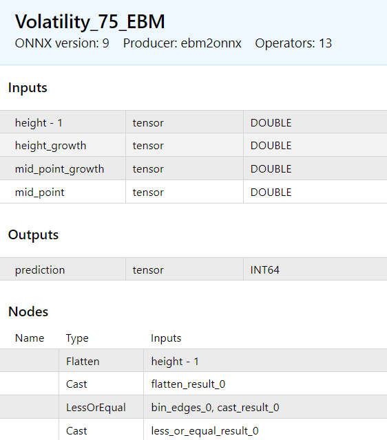
Fig 13: The Inputs and Outputs of our ONNX Model.
We will now create an Expert Advisor and import our ONNX Model.
We start by specifying general file information.
//+------------------------------------------------------------------+
//|                                                         ONNX.mq5 |
//|                                  Copyright 2023, MetaQuotes Ltd. |
//|                                             https://www.mql5.com |
//+------------------------------------------------------------------+
//Meta properties
#property copyright "Gamuchirai Zororo Ndawana"
#property link      "https://www.mql5.com/en/users/gamuchiraindawa"
#property version   "1.00"
From there we need to specify a few global variables.
//Trade Library
#include <Trade\Trade.mqh>           //We will use this library to modify our positions

//Global variables
//Input variables
input double atr_multiple =0.025;    //How many times the ATR should the SL & TP be?
int input lot_mutliple = 1;          //How many time greater than minimum lot should we enter?
const int atr_period = 200;          //ATR Period

//Trading variables
double ask, bid,atr_stop;            //We will use these variables to determine where we should place our ATR
double atr_reading[];                //We will store our ATR readings in this arrays
int    atr;                          //This will be our indicator handle for our ATR indicator
long min_distance;                   //The smallest distance allowed between our entry position and the stop loss
double min_volume;                   //The smallest contract size allowed by the broker
static double initial_balance;       //Our initial trading balance at the beginning of the trading session
double current_balance;              //Our trading balance at every instance of trading
long     ExtHandle = INVALID_HANDLE; //This will be our model's handler
int      ExtPredictedClass = -1;     //This is where we will store our model's forecast
CTrade   ExtTrade;                   //This is the object we will call to open and modify our positions

//Reading our ONNX model and storing it into a data array
#resource "\\Files\\Volatility_75_EBM.onnx" as uchar ExtModel[] //This is our ONNX file being read into our expert advisor

//Custom keyword definitions
#define  PRICE_UP 1
#define  PRICE_DOWN 0
From there we specify the OnInit() Function. We use the OnInit function to setup our ONNX model. To setup or ONNX model we simply need to complete 3 easy steps. We first create the ONNX model from the buffer we used in our global variables above when we required the ONNX model as a resource. After reading it in we need to specify the shape of each individual input, then we specify the shape of each individual output. After doing so, we check if any errors were thrown when we tried to set the input and output shape. If everything went well, we proceed to also fetch the minimum contract volume allowed by our broker, the minimum distance between the stop loss and the entry position and we also setup our ATR indicator.
int OnInit()
  {
   //Check if the symbol and time frame conform to training conditions
   if(_Symbol != "Volatility 75 Index" || _Period != PERIOD_M1)
       {
            Comment("Model must be used with the Volatility 75 Index on the 1 Minute Chart");
            return(INIT_FAILED);
       }

    //Create an ONNX model from our data array
    ExtHandle = OnnxCreateFromBuffer(ExtModel,ONNX_DEFAULT);
    Print("ONNX Create from buffer status ",ExtHandle);

    //Checking if the handle is valid
    if(ExtHandle == INVALID_HANDLE)
      {
            Comment("ONNX create from buffer error ", GetLastError());
            return(INIT_FAILED);
      }

   //Set input shape
   long input_count = OnnxGetInputCount(ExtHandle);
   const long input_shape[] = {1};
   Print("Total model inputs : ",input_count);

   //Setting the input shape of each input
   OnnxSetInputShape(ExtHandle,0,input_shape);
   OnnxSetInputShape(ExtHandle,1,input_shape);
   OnnxSetInputShape(ExtHandle,2,input_shape);
   OnnxSetInputShape(ExtHandle,3,input_shape);

   //Check if anything went wrong when setting the input shape
   if(!OnnxSetInputShape(ExtHandle,0,input_shape) || !OnnxSetInputShape(ExtHandle,1,input_shape) || !OnnxSetInputShape(ExtHandle,2,input_shape) || !OnnxSetInputShape(ExtHandle,3,input_shape))
      {
            Comment("ONNX set input shape error ", GetLastError());
            OnnxRelease(ExtHandle);
            return(INIT_FAILED);
      }

   //Set output shape
   long output_count = OnnxGetOutputCount(ExtHandle);
   const long output_shape[] = {1};
   Print("Total model outputs : ",output_count);
   //Setting the shape of each output
   OnnxSetOutputShape(ExtHandle,0,output_shape);
   //Checking if anything went wrong when setting the output shape
   if(!OnnxSetOutputShape(ExtHandle,0,output_shape))
      {
            Comment("ONNX set output shape error ", GetLastError());
            OnnxRelease(ExtHandle);
            return(INIT_FAILED);
      }
    //Get the minimum trading volume allowed
    min_volume = SymbolInfoDouble(_Symbol,SYMBOL_VOLUME_MIN);
    //Symbol information
    //The smallest distance between our point of entry and the stop loss
    min_distance = SymbolInfoInteger(_Symbol,SYMBOL_TRADE_STOPS_LEVEL);
    //Initial account balance
    initial_balance = AccountInfoDouble(ACCOUNT_BALANCE);
    //Setting up our ATR indicator
    atr = iATR(_Symbol,PERIOD_CURRENT,atr_period);
    return(INIT_SUCCEEDED);
//---
  }
The DeInit function is very simple, it removes the ONNX handler so that we don't tie up resources we aren't using.
void OnDeinit(const int reason)
  {
//---
   if(ExtHandle != INVALID_HANDLE)
      {
         OnnxRelease(ExtHandle);
         ExtHandle = INVALID_HANDLE;
      }
  }
The OnTick function is the heart of our Expert Advisor, it is called every time we receive a new tick from our broker. In our case, we start of by keeping track of time, this allows us to separate processes that we want to perform on every tick and processes that we want to perform whenever a new candle has formed. We want to update our bid and ask prices every tick, we also want to update our take profit and stop loss positions on every tick, however we only want to make a model forecast once on a new candle has formed if we don't have any open positions.
void OnTick()
  {
//---
   //Time trackers
   static datetime time_stamp;
   datetime time = iTime(_Symbol,PERIOD_M1,0);

   //Current bid price
   bid = SymbolInfoDouble(_Symbol,SYMBOL_BID);
   //Current ask price
   ask = SymbolInfoDouble(_Symbol,SYMBOL_ASK);

   //Copy the ATR reading our array for storing the ATR value
   CopyBuffer(atr,0,0,1,atr_reading);

   //Set the array as series so the natural time ordering is preserved
   ArraySetAsSeries(atr_reading,true);

   //Calculating where to position our stop loss
   //For now we'll keep it simple, we'll add the minimum volume and the current ATR reading and multiply it by the ATR multiple
   atr_stop = ((min_distance + atr_reading[0]) * atr_multiple);

   //Current Session Profit and Loss Position
   current_balance = AccountInfoDouble(ACCOUNT_BALANCE);
   Comment("Current Session P/L: ",current_balance - initial_balance);

   //If we have a position open we need to update our stoploss
   if(PositionsTotal() > 0){
        check_atr_stop();
   }

    //Check new bar
     if(time_stamp != time)
      {
         time_stamp = time;

         //If we have no open positions let's make a forecast and open a new position
         if(PositionsTotal() == 0){
            Print("No open positions making a forecast");
            PredictedPrice();
            CheckForOpen();
         }
      }

  }
From there we define the function that will update our ATR take profit and stop loss position. The function iterates over every position we have open and checks if the position matches the symbol we're trading. If it does it then fetches more information about the position, from there it adjusts the position's stop loss and take profit accordingly depending on the direction of the position. Note that, if the trade is moving against our position, it will leave the take profit and stop loss wherever they are.
//--- Functions
//This function will update our S/L & T/P based on our ATR reading
void check_atr_stop(){

      //First we iterate over the total number of open positions
      for(int i = PositionsTotal() -1; i >= 0; i--){

            //Then we fetch the name of the symbol of the open position
            string symbol = PositionGetSymbol(i);

            //Before going any further we need to ensure that the symbol of the position matches the symbol we're trading
                  if(_Symbol == symbol){
                           //Now we get information about the position
                           ulong ticket = PositionGetInteger(POSITION_TICKET); //Position Ticket
                           double position_price = PositionGetDouble(POSITION_PRICE_OPEN); //Position Open Price
                           long type = PositionGetInteger(POSITION_TYPE); //Position Type
                           double current_stop_loss = PositionGetDouble(POSITION_SL); //Current Stop loss value

                           //If the position is a buy
                           if(type == POSITION_TYPE_BUY){
                                  //The new stop loss value is just the ask price minus the ATR stop we calculated above
                                  double atr_stop_loss = (ask - (atr_stop));
                                  //The new take profit is just the ask price plus the ATR stop we calculated above
                                  double atr_take_profit = (ask + (atr_stop));

                                  //If our current stop loss is less than our calculated ATR stop loss
                                  //Or if our current stop loss is 0 then we will modify the stop loss and take profit
                                 if((current_stop_loss < atr_stop_loss) || (current_stop_loss == 0)){
                                       ExtTrade.PositionModify(ticket,atr_stop_loss,atr_take_profit);
                                 }
                           }

                            //If the position is a sell
                           else if(type == POSITION_TYPE_SELL){
                                     //The new stop loss value is just the bid price plus the ATR stop we calculated above
                                     double atr_stop_loss = (bid + (atr_stop));
                                     //The new take profit is just the bid price minus the ATR stop we calculated above
                                     double atr_take_profit = (bid - (atr_stop));

                                 //If our current stop loss is greater than our calculated ATR stop loss
                                 //Or if our current stop loss is 0 then we will modify the stop loss and take profit
                                 if((current_stop_loss > atr_stop_loss) || (current_stop_loss == 0)){
                                       ExtTrade.PositionModify(ticket,atr_stop_loss,atr_take_profit);
                                 }
                           }
                  }
            }
}
We also need another function to open a new position. Note that we use the global bid and ask variables we declared above. This ensures that the entire program is using the same price. Furthermore, we set out stop loss and take profit both to 0 because that will be managed by our check_atr_stop function.
void CheckForOpen(void)
   {
      ENUM_ORDER_TYPE signal = WRONG_VALUE;

      //Check signals
      if(ExtPredictedClass == PRICE_DOWN)
         {
            signal = ORDER_TYPE_SELL;
         }
      else if(ExtPredictedClass == PRICE_UP)
         {
            signal = ORDER_TYPE_BUY;
         }

      if(signal != WRONG_VALUE && TerminalInfoInteger(TERMINAL_TRADE_ALLOWED))
         {
            double price, sl = 0 , tp = 0;

            if(signal == ORDER_TYPE_SELL)
               {
                  price = bid;
               }

           else
               {
                  price = ask;
               }

            Print("Opening a new position: ",signal);
            ExtTrade.PositionOpen(_Symbol,signal,min_volume,price,0,0,"ONNX Order");
         }
   }
Lastly, we need a function to make predictions using our ONNX model inside our expert advisor. The function will also be responsible for preprocessing our data in the same manner it was preprocessed during training. This point cannot be stressed enough, care must be taken to ensure that the data is processed in a consistent manner in training and in production. Note that each input to the model is stored in its own vector, and each vector is then passed to the ONNX Run function in the same order they were passed to the model during training. It is paramount that we maintain consistency through the entire project, otherwise we may experience runtime errors that may not throw any exceptions when we compile our model. Make sure the datatype of each input vector matches the input type the model is expecting and furthermore the output type should match the model's output type.
void PredictedPrice(void)
   {
      long output_data[] = {1};

      double lag_2_open = double(iOpen(_Symbol,PERIOD_M1,3));
      double lag_2_high = double(iOpen(_Symbol,PERIOD_M1,3));
      double lag_2_close = double(iClose(_Symbol,PERIOD_M1,3));
      double lag_2_low = double(iLow(_Symbol,PERIOD_M1,3));
      double lag_2_mid_point = double((lag_2_high + lag_2_low) / 2);
      double lag_2_height = double(( lag_2_mid_point - lag_2_close));

      double lag_open = double(iOpen(_Symbol,PERIOD_M1,2));
      double lag_high = double(iOpen(_Symbol,PERIOD_M1,2));
      double lag_close = double(iClose(_Symbol,PERIOD_M1,2));
      double lag_low = double(iLow(_Symbol,PERIOD_M1,2));
      double lag_mid_point = double((lag_high + lag_low) / 2);
      double lag_height = double(( lag_mid_point - lag_close));

      double   open  =  double(iOpen(_Symbol,PERIOD_M1,1));
      double   high  = double(iHigh(_Symbol,PERIOD_M1,1));
      double   low   = double(iLow(_Symbol,PERIOD_M1,1));
      double   close = double(iClose(_Symbol,PERIOD_M1,1));
      double   mid_point = double( (high + low) / 2 );
      double   height =  double((mid_point - close));

      double first_height_delta = (height - lag_height);
      double second_height_delta = (lag_height - lag_2_height);
      double height_growth = first_height_delta - second_height_delta;

      double first_midpoint_delta = (mid_point - lag_mid_point);
      double second_midpoint_delta = (lag_mid_point - lag_2_mid_point);
      double mid_point_growth = first_midpoint_delta - second_midpoint_delta;

      vector input_data_lag_height = {lag_height};
      vector input_data_height_grwoth = {height_growth};
      vector input_data_midpoint_growth = {mid_point_growth};
      vector input_data_midpoint = {mid_point};

       if(OnnxRun(ExtHandle,ONNX_NO_CONVERSION,input_data_lag_height,input_data_height_grwoth,input_data_midpoint_growth,input_data_midpoint,output_data))
         {
            Print("Model Inference Completed Successfully");
            Print("Model forecast: ",output_data[0]);
         }
       else
       {
            Print("ONNX run error : ",GetLastError());
            OnnxRelease(ExtHandle);
       }

       long predicted = output_data[0];

       if(predicted == 1)
         {
            ExtPredictedClass = PRICE_UP;
         }

       else if(predicted == 0)
         {
            ExtPredictedClass = PRICE_DOWN;
         }
   }
Once that is done, we are ready to compile our model and forward test it using a demo account on our MetaTrader 5 Terminal.
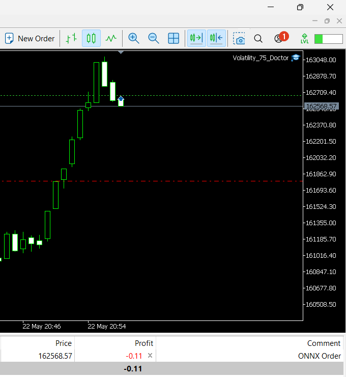
Fig 14: Forward testing our Glass-box ONNX Expert Advisor
Ensure that your model is running without any errors by checking the experts tab and the journal tab.
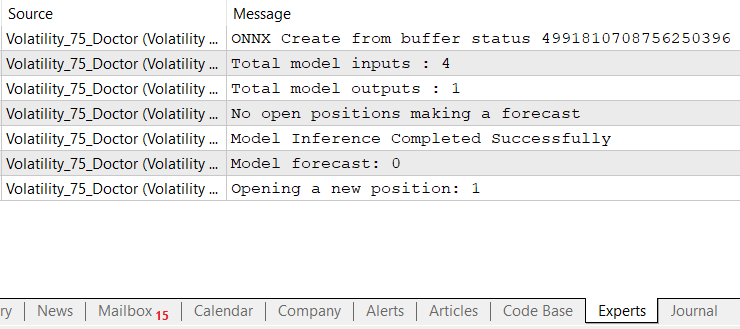
Fig 15: Checking For Any Errors in The Experts Tab
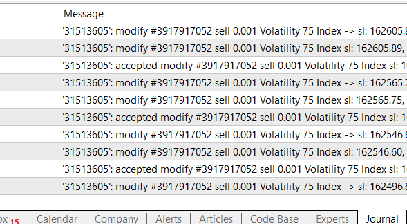
Fig 16: Checking for errors in the journal tab
As we can see the model is running fine. Remember that we can adjust the advisor's settings at any time we want.
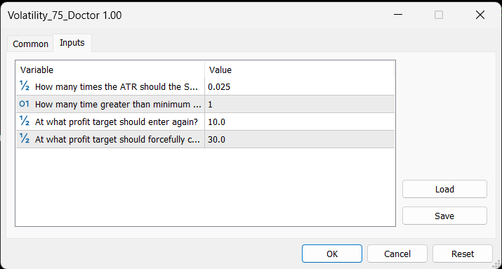
Fig 17: Adjusting the Expert Advisor's Settings
Frequently Encountered Challenges
In this section of the article, we’ll recreate some of the errors one may encounter when first getting setup. We’ll examine what is causing the error and finally go over one solution for each issue.
Failing to Correctly Set Input or Output Shapes.
The most encountered problem is caused by failing to set the input our output shape correctly, remember that you must define the input shape for each feature your model is expecting. Ensure that you iterate through each index and define the input shape for each feature at that index. If you fail to specify the shape for each feature your model may still compile without throwing any errors as shown in the demonstration below, however when we attempt to perform inferencing with the model the error will be uncovered. The error code is 5808, and the MQL5 documentation describes it as “Tensor dimension not set or invalid”. Remember we have 4 inputs in this example however in the code example below we are only setting one input shape.
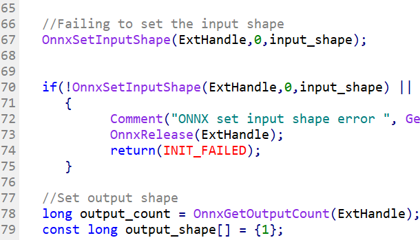
Fig 18: The Expert Advisor Compiles Without Throwing Any Exceptions
We have also included a screenshot of what the error looks like when you inspect your "Experts" tab and remember that the correct code has been attached to the article.

Fig 19: Error Message 5808
Incorrect Typecasting
Incorrect typecasting may sometimes result in total loss of data, or the Expert Advisor will simply crash. In the example below we used an integer array to store the output of our ONNX model, remember our ONNX model has output of type int64. Why do you think this will throw an error? This causes an error because the int type does not have enough memory to store our model’s output causing the model to fail. Our model output requires 8 bytes but our int array only provides 4. The solution is simple, ensure that you are using the right datatype to store your inputs and outputs and if you must typecast ensure you are conforming to the typecasting rules specified in the MQL5 documentation. The error code is 5807 and the description is “Invalid parameter size.”

Fig 20: Incorrect Typecasting

Fig 21: Error Message 5807
Failing To Call ONNX Run
The ONNX Run function expects each of the model inputs to be passed in its own array, separately. In the code example below, we joined all the inputs into one array, and we’re passing that single array to the ONNX Run function. This doesn’t raise any exceptions when we compile the code, however upon execution it will throw an error in the Expert Tab. The error code is 5804 and the documentation concisely describes it as “Invalid number of parameters passed to OnnxRun”.

Fig 22: Failing to call the ONNXRun Function.
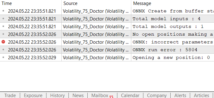
Fig 23: Error Message 5804
Conclusion
To review, you now understand why glass-box models can be useful for us as Financial Engineers, they give us valuable insight with little labor relative to the amount of effort it would've taken to faithfully extract the same information from a black-box model. Furthermore glass-box models are easier to debug, maintain, interpret, and explain. It's not enough for us to assume our models are behaving as we intended, we must validate that they are by looking underneath the hood so to speak.
There is one big disadvantage of glass-box models that we haven't covered till now, they aren't as flexible as black-box models. Glass-box models are an open field of research and as time progresses, we may see more flexible glass-box models in the future, however at the time of this writing they aren't as flexible meaning that there are relationships that may be better modelled by a black-box model. Furthermore, the current implementations of glass box models are based on decision trees, therefore the current implementation of ExplainableBoostingClassifiers in InterpretML inherit all the shortcomings of decision trees.
Until we meet again, I wish you peace, love, harmony and profitable trades.
 Implementation of the Augmented Dickey Fuller test in MQL5
 Data label for time series mining (Part 5):Apply and Test in EA Using Socket
- Free trading apps
- Over 8,000 signals for copying
- Economic news for exploring financial markets
You agree to website policy and terms of use
Awesome thank you , Well explained and clear instructions , Going to see if I can follow your comprehensive instruction, thanks for the ideas .
Great stuff was able to connect to demo acct (only a subset of symbols there expect that is the demo account ) tried one that was there AUDHKD but stuck in disagreement problem line 204 ,
ValueError: at least one array or dtype is required
tried with NZDCNH it seems to work through some iterations but fails in the sklern\multiclass on line 167 with a datahandling
debug tells me valueerror in line 204 one array or dtype is required - in may be I need to check my demo environment as I only created it today :)
on the default Boom1000 Index the problem is line 100 with date and time. raise KeyError(key)
KeyError: 'time' . Possibly an issue as my timezone is New Zealand
Out of time today for testing , will try again tomorrow.Hi Linfo, I hope this helps:
1) The 'time' column was the name my broker gave to a UNIX timestamp that marks each of the rows in the data I fetched. Maybe your broker uses a different name instead, like 'date' is common. Check the dataframe that you get after calling copy_rates_range. The fact that you're getting a "KeyError" thrown, might mean either the dataframe is totally empty or there's no column named 'time' it probably has a different name on your side.
2) Validate the output from copy_rates_range,from what you've described I think that's where things may be falling apart. Check the column names of the data that's being returned to you after making the call.
If these steps don't work let me know.
Thank you for the prompt feedback and advice .
Updating here as it may be useful to others . My issues ;
1) I set up a new demo account to test this and not all currencies where available to This is resolved by opening the acct and ensuring the currencies you want are active (gold colored)
2)There was no Boom1000 Index (data) provided to me by the server , it was in the list but I not against my account (ensure you change the default to be something you have access to and that can give a result) .
3) For me the interpret results would not show in std python , I could only get working with anaconda installed (It would have been easier if I had installed that first).
After this hiccup the documentation was clear and helpful,I am still digesting the results so far so have not yet moved on to the mql5 side
Thank you again for publishing and I look forward to actually understanding the process better . Regards Neil
I'm glad to see that you're making material progress Neil.
Surprisingly: the most important phrase for understanding the material is at the very end of the article:
текущие реализации моделей стеклянного ящика основаны на деревьях решений
Surprisingly: the most important phrase for understanding the material is at the very end of the article: