Gain An Edge Over Any Market

Contents

1. Synopsis
2. Introduction
3. Overview of the strategy: Alternative data sources
4. Machine learning techniques
5. Building the strategy
6. Conclusion
7. Recommendations

Synopsis

Today, we will craft a robust trading strategy designed to provide traders with a significant competitive advantage across various markets. While conventional market participants solely rely on some combination of price-related data, technical indicators and public news announcements for decision making, our strategy takes a trail-blazing approach by leveraging alternative data sources that remain largely unexplored by the majority.

The premise behind our strategy lies in the integration of alternative data, an option often overlooked by mainstream market participants. By harnessing these untapped data sources and applying machine learning techniques, we may position ourselves to gain unique insights and perspectives that are exclusive to our strategy.

In our exploration, we will examine data provided by the St. Louis Federal Reserve Bank, specifically leveraging their comprehensive econometric time-series database known as FRED. FRED is accessible to the public at all times, and unquestionably offers data crucial for informed decision-making in trading. Furthermore, data sourced from central banks like the St. Louis Fed often serves as leading indicators, enhancing our ability to time entries and exits effectively.

Moreover, this data is immune to external manipulation, making it an ideal candidate for integration into our trading strategy.

This article aims to serve as a practical guide, demonstrating the easy utilization of Python and MetaTrader 5 to construct cutting-edge trading strategies. Our commitment to clarity and simplicity ensures that every aspect is explained clearly, enabling readers to grasp our approach effortlessly and get started today!

Introduction: This article aims to demonstrate how to easily apply alternative data in trading strategies. 

By the end of this article, readers will gain insights into the following key areas:

1. How alternative data can aid decision-making amidst noise and uncertainty.
2. Techniques for screening and identifying reliable sources of alternative data.
3. Best practices for analyzing and preprocessing alternative data for analysis.
4. Building robust trading strategies that integrate alternative data sources to enhance the decision-making process.

One example illustrating the impact of alternative data is the strategic use of satellite imagery. Advanced traders leverage satellite images to monitor shipping traffic patterns or observe the inventory levels of oil tankers. These unique data points enable traders to uncover profitable trading opportunities that might otherwise remain hidden.

While the use of satellite imagery may be more common among affluent traders, this article shows how any trader can employ freely available alternative data to stay ahead of the market. Additionally, by using machine learning models, we can analyze multiple data sources simultaneously, further enhancing their decision-making capabilities.

Overview of the Trading Strategy: Alternative Data Sources

Our trading strategy is designed to be easily understandable. We will integrate conventional market data from our MetaTrader 5 Terminal with alternative data sourced from the St. Louis Federal Reserve Bank, specifically focusing on forecasting the future price movements of the GBPUSD pair.

To achieve this, we will leverage two key economic datasets as our alternative data sources. The first dataset provides information on the Great British Pound, offering a time-series of interest rates charged for off-hour bank transactions in the British Sterling Market. These interest rate fluctuations serve as a proxy for gauging the level institutional demand for Sterling, providing valuable indicators for our forecasting models.

Similarly, the second dataset has information on the United States Dollar and comprises a time-series of interest rates charged for overnight loans to American banks, governed by the Federal Reserve. The Federal Reserve's control over these interest rates through monetary policy adjustments offers alternative insights into economic trends that may impact the USD.

By analyzing and interpreting these economic time-series data and employing machine learning techniques, we may hopefully realize our goal of uncovering leading indicators that grant us a competitive advantage in the market.

The cornerstone of our strategy's effectiveness depends on securing a dependable source of alternative data. The availability of reliable alternative data sources varies depending on the markets in which you trade. Synthetic markets, generated by random number generators, have practically no alternative data sources. This is because synthetic markets are independent of the outside world.

1. Credibility: How does your source of alternative data get the data in the first place? Examine the reliability of the information channels they depend on. Questions such as 'How do they access their information?' and 'Are their channels of information trustworthy?' are crucial in assessing credibility. Any doubts regarding these aspects signal the need for a more thorough evaluation.
2. Frequency of Updates: Our focus lies on alternative data sources updated daily, aligning with our trading time frame. However, it's vital to note that not all sources offer daily updates; some may be updated monthly or annually.Therefore be sure to choose a source that aligns with your desired trading frequency.
3. Reputation: Beyond credibility, prioritise sources with a reputable track record and a proven interest in maintaining accuracy. A reputable provider not only adds credibility to our data but also demonstrates accountability.
4. Transparent Presentation: Opt for providers who present data transparently and in a user-friendly manner. Clarity and simplicity in data presentation are paramount for effective decision-making, especially considering the cognitive load associated with complex data.
5. Pricing Structure: Evaluate the pricing models of alternative data sources, balancing our needs and budget constraints. While some sources may be free, others may require payment. Our choice should align with the value proposition offered by each source.
6. Terms and Conditions: Carefully review and understand the terms and conditions associated with alternative data sources, particularly those requiring payment. Clear comprehension of usage restrictions and limitations ensures informed decision-making and prevents any unintended compliance issues.

In summary, a rigorous assessment of alternative data sources based on credibility, update frequency, reputation, transparency, pricing, and terms and conditions is essential to leverage data effectively within our trading strategy.

We will now begin to examine some alternative data sourced from the St Louis Federal Reserve Bank. There are 2 ways to fetch data from the St Louis Fed:

1. Programmatically Using the FRED Python Library
2. Manually on the FRED Website 

If this is your first time using these datasets, I'd advise you first collect the data manually. This is advisable because the FRED website has useful notes and information regarding each dataset, how it was recorded, what the data represents, whether or not it is seasonally adjusted, the units and scales of measurements and other details of that nature. Once you are familiar with the nature of the data, then you may move on to collecting it programmatically. So, for our first demonstration the datasets were downloaded manually from the St Louis Federal Reserve Website. We will move on to the programmatic approach when we are building the strategy. 

The first thing we will do is collect market data from our MetaTrader 5 using an MQL5 script, I prefer collecting the data this way because you can perform any preprocessing you need on the MQL5 side where you have unlimited access to data. Our script is modestly simple.

• We start by declaring handlers for our technical indicators, we will use 4 moving averages.
• Then we declare buffers to store the readings of our moving averages, the buffers in our case are dynamic arrays.
• Moving on, we then need a name for our file, ours will be the name of the pair we are trading followed by the string "Market Data As Series", and it will be of CSV format.
• Subsequently we declare how much data we would like to collect. 
• Note that the script works with the current time frame of the chart it is applied to.
• We have now arrived at our OnStart() event handler, this is where the heart of our script lies.
• We start by initializing all 4 of our technical indicators.
• Then we copy the indicator values to the arrays we created earlier.
• Once that is done, we then create a file handler to create, write and close our file.
• We then use a simple for loop to iterate through the arrays and write them out to our CSV file. Note that on the first iteration of our loop, we write the column headers, afterwards we write out the actual values we want.
• Once the loop is completed, we close our file, using the file handler and we are now ready to merge the data from our MetaTrader 5 terminal with our alternative data.

#property copyright "Gamuchirai Zororo Ndawana"
#property link      "https://www.mql5.com"
#property version   "1.00"

//---Our handlers for our indicators
int ma_handle_5;
int ma_handle_15;
int ma_handle_30;
int ma_handle_150;

//---Data structures to store the readings from our indicators
double ma_reading_5[];
double ma_reading_15[];
double ma_reading_30[];
double ma_reading_150[];

//---File name
string file_name = _Symbol + " " + " Market Data As Series.csv";

//---Amount of data requested
int size = 1000000;
int size_fetch = size + 100;

void OnStart()
  {
      //---Setup our technical indicators
      ma_handle_5 = iMA(_Symbol,PERIOD_CURRENT,5,0,MODE_EMA,PRICE_CLOSE);
      ma_handle_15 = iMA(_Symbol,PERIOD_CURRENT,15,0,MODE_EMA,PRICE_CLOSE);
      ma_handle_30 = iMA(_Symbol,PERIOD_CURRENT,30,0,MODE_EMA,PRICE_CLOSE);
      ma_handle_150 = iMA(_Symbol,PERIOD_CURRENT,150,0,MODE_EMA,PRICE_CLOSE);
      
      //---Copy indicator values
      CopyBuffer(ma_handle_5,0,0,size_fetch,ma_reading_5);
      ArraySetAsSeries(ma_reading_5,true);
      CopyBuffer(ma_handle_15,0,0,size_fetch,ma_reading_15);
      ArraySetAsSeries(ma_reading_15,true);
      CopyBuffer(ma_handle_30,0,0,size_fetch,ma_reading_30);
      ArraySetAsSeries(ma_reading_30,true);
      CopyBuffer(ma_handle_150,0,0,size_fetch,ma_reading_150);
      ArraySetAsSeries(ma_reading_150,true);

      //---Write to file
       int file_handle=FileOpen(file_name,FILE_WRITE|FILE_ANSI|FILE_CSV,",");
       
    for(int i=-1;i<=size;i++){
      if(i == -1){
            FileWrite(file_handle,"Time","Open","High","Low","Close","MA 5","MA 15","MA 30","MA 150");
      }
      
      else{
            FileWrite(file_handle,iTime(_Symbol,PERIOD_CURRENT,i),
                                 iOpen(_Symbol,PERIOD_CURRENT,i),
                                 iHigh(_Symbol,PERIOD_CURRENT,i),
                                 iLow(_Symbol,PERIOD_CURRENT,i),
                                 iClose(_Symbol,PERIOD_CURRENT,i),
                                 ma_reading_5[i],
                                 ma_reading_15[i],
                                 ma_reading_30[i],
                                 ma_reading_150[i]
                                 );
      } 
    }
  }
//+------------------------------------------------------------------+

We are now ready to start exploring our alternative data alongside our market data.

As always, we will begin by first importing the necessary packages.

import pandas as pd
import numpy as np 
import matplotlib.pyplot as plt
import seaborn as sns

Now we read in the data we exported from our MQL5 script.

GBPUSD = pd.read_csv("C:\\Enter\\Your\\Path\\Here\\MetaQuotes\\Terminal\\NVUSDVJSNDU3483408FVKDL\\MQL5\\Files\\GBPUSD Market Data As Series.csv")

When preparing market data for machine learning, make sure today's price is last and the oldest price is first. 

GBPUSD = GBPUSD[::-1]

Then we need to reset the index.

GBPUSD.reset_index(inplace=True)

Let's define how far ahead we would like to forecast.

look_ahead = 30
splits = 30

We now need to prepare the target. 

GBPUSD["Target"] = GBPUSD["Close"].shift(-look_ahead)
GBPUSD.dropna(inplace=True)

Now we need to make the date the index, this will help us easily align our market data with our alternative data later on.

GBPUSD["Time"] = pd.to_datetime(GBPUSD["Time"])
GBPUSD.set_index("Time",inplace=True)

The first alternative data set we will consider is the Daily Sterling Overnight Index Average (SOIA). It is the average of interest rates charged to banks to borrow Sterlings outside of normal baking hours.

If the average interest rates on Sterlings is rising whilst the average interest rates on the Dollar is falling, that may potentially signal GBP getting stronger than the USD on an institutional level. 

SOIA = pd.read_csv("C:\\Enter\\Your\\Path\\Here\\Downloads\\FED Data\\Daily Sterling Overnight Index Average\\IUDSOIA.csv")

Let's clean up the alternative data. First make the date column a date object.

SOIA["DATE"] = pd.to_datetime(SOIA["DATE"])

Our dataset contains dots, this is presumably meant to represent missing observation. We will replace all the dots with zeros, then replace the zeros with the average value of the column. 

SOIA["IUDSOIA"] = SOIA["IUDSOIA"].replace(".","0")
SOIA["IUDSOIA"] = pd.to_numeric(SOIA["IUDSOIA"])
non_zero_mean = SOIA.loc[SOIA['IUDSOIA'] != 0, 'IUDSOIA'].mean()
SOIA['IUDSOIA'] = SOIA['IUDSOIA'].replace(0, non_zero_mean)

Next we make the date the index.

SOIA.set_index("DATE",inplace=True)

The next source of alternative data we will consider will be the Secured Overnight Financing Rate (SOFR). It is the cost of secured overnight loans, and it is published Daily by the New York Federal Reserve Bank. 

SOFR = pd.read_csv("C:\\Enter\\Your\\Path\\Here\\Downloads\\FED Data\\Secured Overnight Financing Rate\\SOFR.csv")

Please note the preprocessing steps applied to the SOFR dataset are identical to the steps applied to the SOIA dataset, therefore, to keep the article easy to read from start to finish we will omit these steps. 

Let's now merge the 3 data frames we have. By setting left_index and right_index to true we are ensuring that both datasets are being aligned only on days we have complete observations for each of them. For example, the GBPUSD dataset has no records over the weekend, therefore all alternative data points observed over the weekend are not included in our final merged data frame. 

merged_df = SOIA.merge(SOFR,left_index=True,right_index=True)
merged_df = merged_df.merge(GBPUSD,left_index=True,right_index=True)

Then we need to reset our index.

merged_df.reset_index(inplace=True)
merged_df.drop(columns=["index"],inplace=True)

Let's define our predictors.

normal_predictors = ['Open', 'High', 'Low', 'Close', 'MA 5', 'MA 15','MA 30', 'MA 150']
alternative_predictors = ['IUDSOIA', 'SOFR']
all_predictors = normal_predictors + alternative_predictors

Then we will create a data frame to store the error levels of each combination of predictors.

accuracy = pd.DataFrame(columns=["Normal","Alternative","All"],index=np.arange(0,splits))

This is what our data frame looks like now.

merged_df

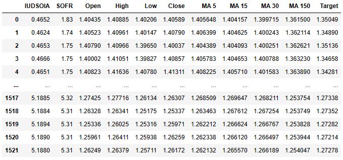
Fig 3: Our dataset that contains both our normal data and our alternative data.

The first column is the average interest rate on the Sterling, the second column contains the average interest rate on the American Dollar. From there the following columns should already be familiar to you. Remember the target is the closing price 30 days into the future.

Lastly we will export our merged data frame to a csv file for later use.

merged_df.to_csv('Alternative Data Target Look Ahead 30.csv')

Let's scale our data.

from sklearn.preprocessing import StandardScaler
scaled_data = merged_df.loc[:,all_predictors]
scaler = StandardScaler()
scaler.fit(scaled_data)
scaled_data = pd.DataFrame(scaler.transform(scaled_data),index=merged_df.index,columns=all_predictors)

Let's now get ready to train our model and see if our alternative data is helping, us or holding us back.

from sklearn.linear_model import LinearRegression
from sklearn.metrics import mean_squared_error 
from sklearn.model_selection import TimeSeriesSplit

Let's prepare our train/test split.

tscv = TimeSeriesSplit(gap=look_ahead+10,n_splits=splits)

for i,(train,test) in enumerate(tscv.split(merged_df)):
    model = LinearRegression()
    model.fit(scaled_data.loc[train[0]:train[-1],all_predictors],merged_df.loc[train[0]:train[-1],"Target"])
    accuracy["All"][i] = mean_squared_error(merged_df.loc[test[0]:test[-1],"Target"],model.predict(scaled_data.loc[test[0]:test[-1],all_predictors]))

Now we are plotting the results as box-plots.

fig,axs = plt.subplots(1,3,sharex=True,sharey=True,figsize=(16,4))

for i,ax in enumerate(axs.flat):
    ax.boxplot(merged_df.iloc[:,i])
    ax.set_title(accuracy.columns[i])

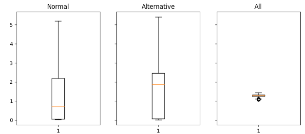
Fig 4: Analyzing the error values we got when using Normal Data (left), Alternative Data (middle), All Available Data (right)

Let's interpret the results: we can clearly see the normal set of predictors and the alternative set of predictors both have long tails that reach towards the top of the plot. However, the last plot, the plot that has both the normal and alternative predictors, has a squashed shape. This squashed shape is desirable because it shows that when we use both sets of predictors together, we get less variation in our errors. Our accuracy is stable in the last plot, however on the first two plots where we either rely totally on normal data or alternative data our accuracy isn't as stable. 

We can also check if there are any interaction effects in our data. We will create a scatter plot of the target on the y-axis and the Sterling Interest rate on the x-axis.

sns.scatterplot(x=merged_df["IUDSOIA"],y=merged_df["Target"])

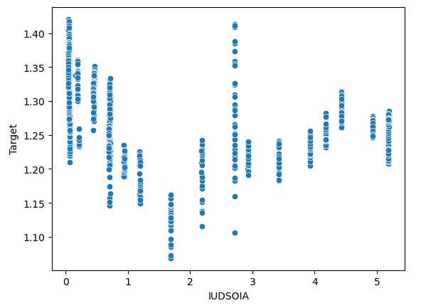
Fig 5: Analyzing the relationship between the Interest rate charged on Sterlings and the future value of the GBPUSD pair.

Here's one way of interpreting this plot, each line running from the top of the plot to the bottom represents how the target changes when the Sterling interest rate is fixed. The fact that we can observe varying target values even though our Sterling Interest rate is fixed is a definite sign of interaction effects in our data. This may be an indicator that there are other powerful forces at play that are influencing the target beyond the alternative data we have collected.

Machine Learning Techniques 

The selection of an appropriate machine learning technique is influenced by the nature of the data you have. Consider the following:

• Dataset Size: For small datasets with fewer than ten thousand rows or less than 30 columns, it's advisable to employ simpler models to mitigate the risk of overfitting. Complex models like deep neural networks may struggle to learn effectively with such limited data.
• Data Noisiness: Noisy datasets, typically this means datasets with missing data points or random unexplained fluctuations, are better suited for simpler models. Complex models tend to exhibit high variance, making them more likely to overfit on noisy data and furthermore on especially noisy market days we may even be better off without them.
• Data Dimensionality: In cases where the dataset has a high number of columns, preprocessing techniques can be beneficial. Employ models that are effective at handling high-dimensional data and apply feature selection and dimensionality reduction.
• Data Size and Computational Power: If you have large datasets with acceptable noise levels and on top of that you also have access to sufficient computational resources, then that may warrant the use of sophisticated models like deep neural networks. These models can effectively capture complex patterns and relationships within the data given adequate computational capabilities and clean data.

In conclusion, there is no perfect solution for machine learning model selection. The nature of the data, including size, noisiness, dimensionality, and available computational power, plays a pivotal role in determining the most suitable approach. Adapting the choice of model to align with the data's characteristics is crucial for achieving robust and accurate predictive outcomes. 
We will now demonstrate how you can select a good model for your data.

We will start by importing the libraries we need.

import statistics as st

import pandas as pd
import numpy as np
import seaborn as sns
import matplotlib.pyplot as plt

from sklearn.linear_model import Lasso,Ridge,LinearRegression
from sklearn.ensemble import RandomForestRegressor
from sklearn.model_selection import TimeSeriesSplit
from sklearn.metrics import mean_squared_error
from sklearn.svm import SVR
from sklearn.preprocessing import StandardScaler

from xgboost import XGBRegressor

Now we will read in the data from the csv we exported. The CSV had all our merged data.

csv = pd.read_csv("C:\\Enter\\Your\\Path\\Here\\Alternative Data.csv")

Let's get ready to scale the data.

predictors = ['IUDSOIA', 'SOFR', 'Open', 'High', 'Low', 'Close']
target = 'Target'
scaled_data = csv.loc[:,predictors]
scaler = StandardScaler()
scaler.fit(scaled_data)
scaled_data = scaler.transform(scaled_data)

Let's train our models.

splits = 10
gap = 30
models = ['Linear','Lasso','Ridge','Random Forest','Linear SVR','Sigmoid SVR','RBF SVR','2 Poly SVR','3 Poly SVR','XGB']

Let's prepare our train/test split and then let's create a data frame to store the error metrics.

tscv = TimeSeriesSplit(n_splits=splits,gap=gap)
error_df = pd.DataFrame(index=np.arange(0,splits),columns=models)

Now we can observe our model's error metrics.

for i,(train,test) in enumerate(tscv.split(csv)):
    model=XGBRegressor()
    model.fit(scaled_data.loc[train[0]:train[-1],predictors],csv.loc[train[0]:train[-1],target])
    error_df.iloc[i,9] =mean_squared_error(csv.loc[test[0]:test[-1],target],model.predict(scaled_data.loc[test[0]:test[-1],predictors]))

error_df

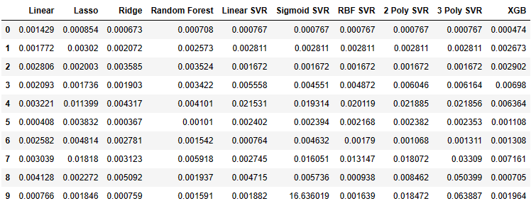
Fig 6: The error values we received from each of the model's we fit.

Let's visualize some of the data as boxplots.

fig , axs = plt.subplots(2,5,figsize=(20,20),sharex=True)

for i,ax in enumerate(axs.flat):
    ax.boxplot(error_df.iloc[:,i])
    ax.set_title(error_df.columns[i])

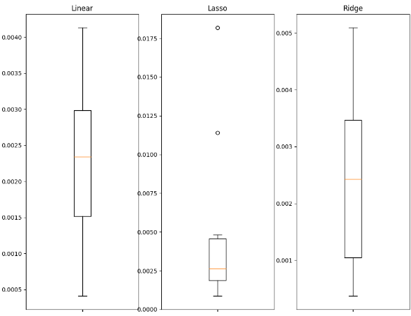
Fig 7: The error values of some of the linear models we used.

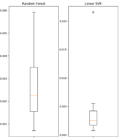
Fig 8: The error values of some of the non-linear models we used.

We will display some of the summary statistics obtained.

Variance	Error
Linear variance: 1.3365981802501968e-06	Linear mean squared error: 0.0022242681292296462
Lasso variance: 3.0466413126186177e-05	Lasso mean squared error: 0.004995731270431843
Ridge variance: 2.5678314939547713e-06	Ridge mean squared error: 0.002467126140156681
Random Forest variance: 2.607918492340197e-06	Random Forest mean squared error: 0.002632579355696408
Linear SVR variance: 3.825627012092798e-05	Linear SVR mean squared error: 0.004484702122899226
Sigmoid SVR variance: 27.654341711864102	Sigmoid SVR mean squared error: 1.6693947903605928
RBF SVR variance: 4.1654658535332505e-05	RBF SVR mean squared error: 0.004992333849448852
2 Poly SVR variance: 6.739873404310582e-05	2 Poly SVR mean squared error: 0.008163708245600027
3 Poly SVR variance: 0.0005393054392191576	3 Poly SVR mean squared error: 0.018431036676781344
XGB variance: 7.053078880392137e-06	XGB mean squared error: 0.003163819414983548

Observe that none of the models are performing outstandingly well, they are all more or less within the same band of performance. In such circumstances, the simpler model may be the best choice because it is less likely to be overfitting. Therefore, in this example we will use the linear regression as our model of choice for our trading strategy. We opt for it because its error level is just as good as any other model, we could've chosen and furthermore, its variance is low. So, the linear model is less likely to be overfitting and more likely to be stable overtime. 

Building The Strategy 

We are now ready to apply everything would've discussed in the previous sections into a robust trading strategy using the MetaTrader 5 Library for Python. 

Explanations will be given at every step of the way to ensure all the code is easy to follow.

First we import the packages we need.

from fredapi import Fred
import MetaTrader5 as mt5
import pandas as pd
import numpy as np
import time
from datetime import datetime
import matplotlib.pyplot as plt

The fredapi package allows us to pull data programmatically from the FRED database. However before you can use the library, you must create an API key. API key's are free to create, but you can only obtain one after creating a free user account with the St Louis Fed.

Now we'll define global variables.

LOGIN = ENTER_YOUR_LOGIN
PASSWORD = 'ENTER_YOUR_PASSWORD'
SERVER = 'ENTER_YOUR_SERVER'
SYMBOL = 'GBPUSD'
TIMEFRAME = mt5.TIMEFRAME_D1
DEVIATION = 1000
VOLUME = 0
LOT_MULTIPLE = 1
FRED = Fred(api_key='ENTER_YOUR_API_KEY')

Now we will log in to our trading account.

if mt5.initialize(login=LOGIN,password=PASSWORD,server=SERVER):
    print('Logged in successfully')
else:
    print('Failed To Log in')

Logged in successfully

Let's define our trading volume.

for index,symbol in enumerate(mt5.symbols_get()):
    if symbol.name == SYMBOL:
        print(f"{symbol.name} has minimum volume: {symbol.volume_min}")
        VOLUME = symbol.volume_min * LOT_MULTIPLE

GBPUSD has minimum volume: 0.01

Let's define functions we are going to use throughout our program.

First we need a function to fetch the current market price from our MetaTrader 5 Terminal.

def get_prices():
    start = datetime(2024,3,20)
    end   = datetime.now()
    data  = pd.DataFrame(mt5.copy_rates_range(SYMBOL,TIMEFRAME,start,end))
    data['time'] = pd.to_datetime(data['time'],unit='s')
    data.set_index('time',inplace=True)
    return(data.iloc[-1,:])

Next we need a function to request alternative data from the St Louis Federal Reserve.

def get_alternative_data():
    SOFR = FRED.get_series_as_of_date('SOFR',datetime.now())
    SOFR = SOFR.iloc[-1,-1]
    SOIA = FRED.get_series_as_of_date('IUDSOIA',datetime.now())
    SOIA = SOIA.iloc[-1,-1]
    return(SOFR,SOIA)

Then we need a function to prepare inputs for our model.

def get_model_inputs():
    LAST_OHLC = get_prices()
    SOFR , SOIA = get_alternative_data()
    MODEL_INPUT_DF = pd.DataFrame(index=np.arange(0,1),columns=predictors)
    MODEL_INPUT_DF['Open'] = LAST_OHLC['open']
    MODEL_INPUT_DF['High'] = LAST_OHLC['high']
    MODEL_INPUT_DF['Low'] =  LAST_OHLC['low']
    MODEL_INPUT_DF['Close'] = LAST_OHLC['close']
    MODEL_INPUT_DF['IUDSOIA'] = SOIA
    MODEL_INPUT_DF['SOFR'] = SOFR
    model_input_array = np.array([[MODEL_INPUT_DF.iloc[0,0],MODEL_INPUT_DF.iloc[0,1],MODEL_INPUT_DF.iloc[0,2],MODEL_INPUT_DF.iloc[0,3],MODEL_INPUT_DF.iloc[0,4],MODEL_INPUT_DF.iloc[0,5]]])
    return(model_input_array,MODEL_INPUT_DF.loc[0,'Close'])

Then we need a function to help us make a forecast using our model.

def ai_forecast():
    model_inputs,current_price = get_model_inputs()
    prediction = model.predict(model_inputs)
    return(prediction[0],current_price)

Let's train our model.

training_data = pd.read_csv('C:\\Enter\\Your\\Path\\Here\\Alternative Data.csv')

Setting up our model.

from sklearn.linear_model import LinearRegression
model = LinearRegression()

Defining our predictors and target.

predictors = ['Open','High','Low','Close','IUDSOIA','SOFR']
target     = 'Target'

Fitting our model.

model.fit(training_data.loc[:,predictors],training_data.loc[:,target])

Now we have arrived at the heart of our trading algorithm,

• First we define an infinite loop to keep our strategy up and running.
• Next we fetch current market data and use it to perform a forecast.
• Afterwards we will have boolean flags to represent our model's expectations. If our model is expecting price to rise, BUY_STATE is True otherwise if our model is expecting price to fall, SELL_STATE is false.
• If we have no open positions we will follow our model's forecast.
• If we have open positions, then we will check if our model's forecast is going against our open position. If it is, then we will close the position. Otherwise, we can leave the position open.
• Lastly after completing all the above steps, we will put the algorithm to sleep for a day and fetch updated data the following day.

while True:
    #Get data on the current state of our terminal and our portfolio
    positions = mt5.positions_total()
    forecast , current_price = ai_forecast()
    BUY_STATE , SELL_STATE = False , False

    #Interpret the model's forecast
    if(current_price > forecast):
        SELL_STATE = True
        BUY_STATE  = False 

    elif(current_price > forecast):
        SELL_STATE = False
        BUY_STATE  = True

    print(f"Current price is {current_price} , our forecast is {forecast}")

    #If we have no open positions let's open them
    if(positions == 0):
        print(f"We have {positions} open trade(s)")
        if(SELL_STATE):
            print("Opening a sell position")
            mt5.Sell(SYMBOL,VOLUME)
        elif(BUY_STATE):
            print("Opening a buy position")
            mt5.Buy(SYMBOL,VOLUME)

    #If we have open positions let's manage them
    if(positions > 0):
        print(f"We have {positions} open trade(s)")
        for pos in mt5.positions_get():
            if(pos.type == 1):
                if(BUY_STATE):
                    print("Closing all sell positions")
                    mt5.Close(SYMBOL)
            if(pos.type == 0):
                if(SELL_STATE):
                    print("Closing all buy positions")
                    mt5.Close(SYMBOL)
    #If we have finished all checks then we can wait for one day before checking our positions again
    time.sleep(24 * 60 * 60)

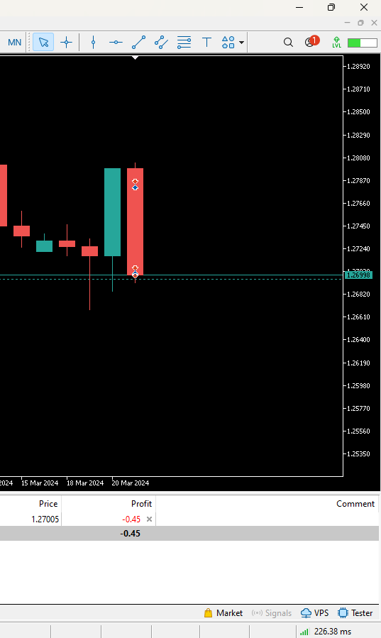
Fig 9: Our trade on the first day we opened it.

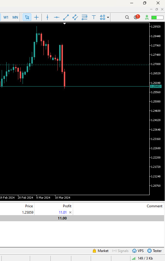
Fig 10: Our trade the following day.

Conclusion 

Alternative data holds vast potential to change the way we look at financial markets. By carefully picking the right sources of data we may potentially find ourselves on the right side of most of the trades we enter. The most important component of this strategy is having a reliable source of alternative data, otherwise you may just as well use normal data. Take your time and do your own research, arrive at your own conclusions and follow your instincts. Remember that at the end of the day, building strategies is as much a science as it is an art.  Therefore, apply your reasoning skills judiciously when selecting which alternative data sources would be useful, and furthermore let your imagination find novel applications and use cases most people wouldn't think of, and you will be in a league of your own making. 

Recommendations

Future readers may find it profitable to search for more sources of alternative datasets and use machine learning techniques such as best subset selection to pick useful sources of alternative data. Furthermore, remember that the linear model we used in our demonstration makes strong assumptions about the process that generated the data, if these assumptions are violated then the accuracy of our model will deteriorate over time.