Neural networks made easy (Part 31): Evolutionary algorithms
Dmitriy Gizlyk | 16 December, 2022
Contents
- Introduction
- 1. Basic algorithm construction principles
- 2. Implementation using MQL5
- 3. Testing
- Conclusion
- References
- Programs used in the article
Introduction
We continue to study non-gradient methods for optimizing models. The main advantage of these optimization methods is the ability to optimize models which cannot be optimized using gradient methods. These are the tasks when it is not possible to determine the derivative of the model function, or its calculation is complicated by some factors. In the previous article, we got acquainted with the genetic optimization algorithm. The ideal of this algorithm is borrowed from the natural sciences. Each model weight is represented by a separate gene in the model's genome. The optimization process evaluates a certain population of models initialized randomly. The population has a finite "lifespan". At the end of the epoch, the algorithm selects the "best" representatives of the population, which will give "offspring" for the next epoch. A pair of "parents" for each individual (model in the new population) is chosen randomly. "Parents' genes" are also inherited randomly.
1. Basic algorithm construction principles
As you can see, there is a lot of randomness in the previously considered genetic optimization algorithm. We purposefully select the best representatives from each population, while most of the population is eliminated. So, during the full iteration of the entire population at each epoch, we perform a lot of "useless" work. In addition, the development of the population of models from epoch to epoch in the direction we need depends largely on the factor of chance. Nothing guarantees a directed movement towards the goal.
If we get back to the gradient descent method, that time we purposefully moved towards the anti-gradient at each iteration. This way we minimized the model error. And the model was moving in the required direction. Of course, in order to apply the gradient descent method, we need to analytically determine the derivative of the function at each iteration.
What if we do not have such an opportunity? Can we somehow combine these two approaches?
Let's first recall the geometric meaning of a function derivative. The derivative of a function characterizes the rate of change of the function value at a given point. It is defined as the limit of the ratio of the function value change to the change in its argument when the change in the argument tends to 0. Provided such a limit exists.
This means that in addition to the analytical derivative, we can find its approximation experimentally. To determine the derivative of a function with respect to an argument x experimentally, we need to slightly change the value of the x parameter, with other conditions being equal, and calculate the value of the function. The ratio of the change in the function value to the change in the argument will give us an approximate value of the derivative.
Since our models are non-linear, in order to obtain a better definition of the derivative experimentally, it is recommended to perform the following 2 operations for each argument. In the first case we will add some value and in the second one we will subtract the same value. The average value of two operations will produce a more accurate approximation of the function derivative value with respect to the analyzed argument at a given point.
This approach is often used when assessing the correctness of the output of a derivative model. Evolutionary algorithms also exploit this property. The main idea of evolutionary optimization strategies is to use gradients obtained experimentally to determine the direction for the optimization of model parameters.
But the main problem in using experimental gradients is the need to execute a large number of operations. For example, to determine the influence of one parameter on the model result, we need to take 3 feed forward passes for the model with the same source data. Accordingly, all model parameters are accompanied by a 3-fold increase in the number of iterations.
This is not good, so we need to do something about it.
For example, we can change not one parameter, but, say, two. But in this case, how to determine the influence of each of them how to change the selected parameters - synchronously or not? What if the influence of the selected parameters on the result is not the same and they should be changed with different intensity?
Well, we could say that the processes occurring inside the model were not important to us. We need a model that meets our requirements. It might not be optimal. Anyway, the concept of optimality is the maximum possible satisfaction of all the requirements presented.
In this case, we can look at the model and the set of its parameters as a single whole. We can use some algorithm and change all the parameters of the model at once. The algorithm for changing parameters can be any, for example random distribution.
We will evaluate the impact of changes in the only available way — by testing the model on the training sample. If the new set of parameters has improved the previous result, then we accept it. If the result has become worse, reject it and return to the previous set of parameters. Again and again repeat the loop for new parameters.
Doesn't look like a genetic algorithm? But where is the estimate of the experimental gradient mentioned above?
Let's get closer to the genetic algorithm. We will again use the whole population of models, the effectiveness of which will be tested on some finite training set. But in this case, we will use for all value the parameters that are close in value, in contrast to the genetic algorithm, in which each model was a kind of individual created randomly. In fact, we will take one model and add some random noise to its parameters. The use of random noise will produce a population in which there will not be a single identical model. A small amount of noise will allow us to get the results of all models in the same subspace with a small deviation. This means that the results of the models will be comparable.
![]()
where w' are parameters of the model in population
w are parameters of the source model
ɛ is a random noise.
To evaluate the efficiency of each model from the population, we can use a loss function or a reward system. The choice largely depends on the problem you are solving. Also, we take into account the optimization policy. We minimize the loss function and maximize the total reward. In the practical part of this article, we will maximize the total reward, similar to the process we implemented when solving the reinforcement learning problem.
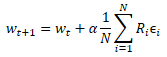
After testing the performance of the new population on the training sample, we need to determine how to optimize the parameters of the original model. If we apply mathematics, we can try to somehow determine the influence of each parameter on the result. Here we will use a number of assumptions. But we agreed earlier to consider the model as a whole. This means that the entire set of noise added in each individual population model can be estimated by the resulting total reward obtained while testing the effectiveness of the model on the training set. Therefore, we will add to the parameters of the original model the weighted average of the corresponding parameter noise from all models of the population. The noise will be weighted by the total reward. And of course, the resulting weighted average will be multiplied by the learning coefficient of the model. The parameter update formula is shown below. As you can see, this formula is very similar to the formula for updating the weights when using gradient descent.
This evolutionary optimization algorithm was proposed by the OpenAI team in September 2017, in the article "Evolution Strategies as a Scalable Alternative to Reinforcement Learning". In the article, the proposed algorithm is considered as an alternative to the previously studied Q-learning and Policy Gradient methods. The proposed algorithm shows good viability and productivity. It also demonstrates tolerance for frequency of action and delayed rewards. In addition, the algorithm scaling method proposed by the authors enables an increase in the problem solving speed with an almost linear dependence, by utilizing additional computing resources. For example, using more than a thousand parallel computers, they managed to solve a 3-dimensional humanoid walking problem in just 10 minutes. But we will not consider the problem of scaling in our article.
2. Implementation using MQL5
We have considered the theoretical aspects of the algorithms, so now let us move on to the practical part, in which we will consider the implementation of the proposed algorithm using MQL5. Please note that the algorithm we are going to implement is not 100% original. There will be some changes, although the entire idea of the algorithm will be preserved. In particular, the authors proposed to use a greedy algorithm for choosing an action. However, we will use a probabilistic algorithm when choosing an action. In addition, we have added mutation parameters, similar to the genetic algorithm. The original algorithm did not use mutation.
To implement the algorithm, let's create a new neural network class CNetEvolution — inherit it from the genetic algorithm model. The inheritance will be private. Therefore, we will need to override all methods used. At first glance, with public inheritance there would be no need to redefine some methods, which we will simply redirect to methods of the parent class. But non-public inheritance will block access to unused methods. This is most useful when overloading methods. The user will not see the overloaded methods of the parent classes, so we avoid unnecessary confusion.
class CNetEvolution : protected CNetGenetic
  {
protected:
   virtual bool      GetWeights(uint layer) override;

public:
                     CNetEvolution() {};
                    ~CNetEvolution() {};
   //---
   virtual bool              Create(CArrayObj *Description, uint population_size) override;
   virtual bool              SetPopulationSize(uint size) override;
   virtual bool              feedForward(CArrayFloat *inputVals, int window = 1, bool tem = true) override;
   virtual bool              Rewards(CArrayFloat *rewards) override;
   virtual bool              NextGeneration(float mutation, float &average, float &mamximum);
   virtual bool              Load(string file_name, uint population_size, bool common = true) override;
   virtual bool              Save(string file_name, bool common = true);
   //---
   virtual bool              GetLayerOutput(uint layer, CBufferFloat *&result) override;
   virtual void              getResults(CBufferFloat *&resultVals);
  };
We do not declare new instances of the class in the new class body. Moreover, we do not declare any internal variables. We will only use objects and variables of parent classes. Therefore, both the constructor and destructor of the class remain empty.
Please note that we do not create objects to store weights of the original model before adding the noise. This is also a deviation from the original algorithm. But we will get back to this issue while implementing the algorithm.
Coming next is the Create method which creates a population of models. The method receives in parameters a dynamic array with the description of one model and the population size, similarly to the parent class methods. The main functionality will be implemented using parent class methods. Here we only need to call the class and to pass the obtained parameters.
In the CNetGenetic::Create genetic algorithm class method, we created a population of models with one architecture and random weights. Now we need to create a similar population. But the parameters of our models should be close. To make them close, we call the NextGeneration method, which we will consider a little later.
Do not forget to check the operation result at each step. At the end of the method, return the logical result of the operations.
bool CNetEvolution::Create(CArrayObj *Description, uint population_size)
  {
   if(!CNetGenetic::Create(Description, population_size))
      return false;
   float average, maximum;
   return NextGeneration(0,average, maximum);
  }
I have earlier mentioned the NextGeneration method. Let's take a look at its algorithm. The functionality of this method is similar to the functionality of the parent class method having the same name. But there are certain specifics associated with the algorithm requirements.
In the parameters, the method receives the probability of mutation and two variables, where we will write the average and maximum rewards.
In the method body, save the required reward values and limit the maximum value of the mutation. We limit the maximum mutation limit because we need to obtain a trained model. If the mutation values are high, we will generate random model parameters at each iteration, regardless of the obtained results. As a consequence, the population will constantly consist of random untrained models.
bool CNetEvolution::NextGeneration(float mutation, float &average, float &maximum)
  {
   maximum = v_Rewards.Max();
   average = v_Rewards.Mean();
   mutation = MathMin(mutation, MaxMutation);
Next, let us prepare the base for updating the model weights. As discussed in the theoretical part of this article, a measure for weighting the noise size when updating parameters is the total reward of an individual model on the training set. But depending on the reward policy used, the total reward can be either positive or negative. With a high degree of probability, we will get a situation where the total rewards of all members of the population will have the same sign. I.e. they will all be either positive or negative.
Not all noise additions to the model parameters have a positive or negative effect. In this case, the positive influence of some components will be covered by the negative influence of others. At best, it will slow down our progress in the right direction. At worst, this may lead the model training in the opposite direction. To minimize the influence of this effect, let's write the difference between the total reward of a particular model and the average total reward of the entire population into the v_Probability vector of probabilities.
This step is connected with the assumption that the noise we are adding belongs to the normal distribution. This means that the total reward of the original model is approximately in the middle of the total distribution of the population's total rewards. Once the difference is calculated, the models with the total reward below the average level will receive a negative probability. The smaller the total reward of the model, the more negative its probability. Likewise, models with the highest total reward will also receive the highest positive probability. What is the practical benefit of it? If the added noise has a positive effect, by multiplying it to a positive probability we shift the weight in the same direction. Thus we encourage the model training in the required direction. If the added noise had a negative effect, then by multiplying it to a negative probability we change the direction of the weight shift from negative to positive. This also directs the model training towards the maximizing of the total reward.
Next, according to the original algorithm, the model parameters are corrected using the weighted average of the noise. Therefore, we also normalize the vector of obtained probabilities to make the sum of the absolute values of all the vector elements equal to 1.
   v_Probability = v_Rewards - v_Rewards.Mean();
   float Sum = MathAbs(v_Probability).Sum();
   if(Sum == 0)
      v_Probability[0] = 1;
   else
      v_Probability = v_Probability / Sum;
After determining the model update coefficients, which we have written in the vectorv_Probability, move on to loop iterating through the model layers. Parameters of new population models will be formed in the body of this loop.
In the loop body, we first get a pointer to a dynamic array of current layer objects. Immediately check the validity of the received pointer. Also, check the size of the dynamic array. It must match the given population size. If the population size is insufficient, call the CreatePopulation method to create additional models. Here we use the parent class method without changes.
   for(int l = 1; l < layers.Total(); l++)
     {
      CLayer *layer = layers.At(l);
      if(!layer)
         return false;
      if(layer.Total() < (int)i_PopulationSize)
         if(!CreatePopulation())
            return false;
After that, call the GetWeights method, which will create the updated parameters of the model's current layer. The parameters will be created in the m_Weights and m_WeightsConv matrices. We will consider the method algorithm later.
      if(!GetWeights(l))
         return false;
After updating the model parameters, we can start populating the population. To do this, let us create a nested loop with the number of iterations equal to the population size.
In the body of the loop, we get a pointer to the object of the current neuron of the neural layer being analyzed. Immediately check the validity of the obtained pointer. Here is also get a pointer to the weight matrix object.
      for(uint i = 0; i < i_PopulationSize; i++)
        {
         CNeuronBaseOCL* neuron = layer.At(i);
         if(!neuron)
           return false;
         CBufferFloat* weights = neuron.getWeights();
If the received weight matrix pointer is valid, then start working with this matrix. Here we create another nested loop that will iterate over the elements of the weight matrix.
In the loop body, we first check the probability of using a mutation and, if necessary, generate a random number. If the generated random number is less than the mutation probability, then write a random weight coefficient into the current element of the matrix. After that move on to the next iteration of the loop. A similar approach was used in the genetic algorithm.
         if(!!weights)
           {
            for(int w = 0; w < weights.Total(); w++)
              {
               if(mutation > 0)
                 {
                  int err_code;
                  float random = (float)Math::MathRandomNormal(0.5, 0.5, err_code);
                  if(mutation > random)
                    {
                     if(!weights.Update(w, GenerateWeight((uint)m_Weights.Cols())))
                       {
                        Print("Error updating the weights");
                        return false;
                       }
                     continue;
                    }
                 }
If the current weight is to be updated, then we first check its current value. If necessary, an invalid number should be replaced with a random weight.
               if(!MathIsValidNumber(m_Weights[0, w]))
                 {
                  if(!weights.Update(w, GenerateWeight((uint)m_Weights.Cols())))
                    {
                     Print("Error updating the weights");
                     return false;
                    }
                  continue;
                 }
At the end of the nested loop iteration, add noise to the current weight.
               if(!weights.Update(w, m_Weights[0, w] + GenerateWeight((uint)m_Weights.Cols())))
                 {
                  Print("Error updating the weights");
                  return false;
                 }
              }
            weights.BufferWrite();
           }
After adding noise to all elements of the weight matrix of the current element of the population, transfer the updated parameters to the OpenCL context memory.
If necessary, repeat the iterations described above for the convolutional layer weight matrix.
         if(neuron.Type() != defNeuronConvOCL)
            continue;
         CNeuronConvOCL* temp = neuron;
         weights = temp.GetWeightsConv();
         for(int w = 0; w < weights.Total(); w++)
           {
            if(mutation > 0)
              {
               int err_code;
               float random = (float)Math::MathRandomNormal(0.5, 0.5, err_code);
               if(mutation > random)
                 {
                  if(!weights.Update(w, GenerateWeight((uint)m_WeightsConv.Cols())))
                    {
                     Print("Error updating the weights");
                     return false;
                    }
                  continue;
                 }
              }

            if(!MathIsValidNumber(m_WeightsConv[0, w]))
              {
               if(!weights.Update(w, GenerateWeight((uint)m_WeightsConv.Cols())))
                 {
                  Print("Error updating the weights");
                  return false;
                 }
               continue;
              }

            if(!weights.Update(w, m_WeightsConv[0, w] + GenerateWeight((uint)m_WeightsConv.Cols())))
              {
               Print("Error updating the weights");
               return false;
              }
           }
         weights.BufferWrite();
        }
     }
Iterations are repeated for all elements of the sequence.
At the end of the method, reset the total reward accumulation vector and terminate the method.
   v_Rewards.Fill(0);
//---
   return true;
  }
According to the sequence of methods, let us now consider the GetWeights method which was called from the previous method. Its purpose is to update the parameters of the model being optimized. The parent genetic algorithm class CNetGenetic had a method of the same name, which was used to download the parameters of one neural layer of all population models. The resulting matrix was then used to create a new population. This time we use the same logic, only the content slightly changes in accordance with the optimization algorithm used.
The method receives in parameters the index of the neural layer for which it is necessary to create a matrix of parameters. In the method body, check the availability of the formed vector with the probabilities of using population representatives when updating the model parameters. Call the parent class method of the same name. Remember to control the execution of operations.
bool CNetEvolution::GetWeights(uint layer)
  {
   if(v_Probability.Sum() == 0)
      return false;
   if(!CNetGenetic::GetWeights(layer))
      return false;
Once the operations of the parent class method are completed, we expect that the m_Weights and m_WeightsConv matrices will contain the weights of the analyzed neural layer for all population models.
Note that the matrices contain weights. However, to update the model parameters, we need the values of the added noise and the parameters of the original model.
We proceed similarly to the adjustment of rewards. We know that noise has a normal distribution. Each parameter of the population models is the sum of the corresponding parameter of the original model and the noise. We make the assumption that the parameters of the original model are in the middle of the distribution of the corresponding parameters of the population models. So, we can use the vector of mean values of the corresponding population parameters.
   if(m_Weights.Cols() > 0)
     {
      vectorf mean = m_Weights.Mean(0);
By subtracting the vector of mean values from the matrix of parameters of the population models, we can find the required matrix of added noise.
      matrixf temp = matrixf::Zeros(1, m_Weights.Cols());
      if(!temp.Row(mean, 0))
         return false;
      temp = (matrixf::Ones(m_Weights.Rows(), 1)).MatMul(temp);
      m_Weights = m_Weights - temp;
If we use the same approach to determine the added noise and the probabilities of its use in updating the model weights, we get comparable values. Next, we can use the above formula for updating model parameters. After that, we only need to transfer the obtained values to the appropriate matrix.
      mean = mean + m_Weights.Transpose().MatMul(v_Probability) * lr;
      if(!m_Weights.Resize(1, m_Weights.Cols()))
         return false;
      if(!m_Weights.Row(mean, 0))
         return false;
     }
If necessary, repeat the operations for the second matrix.
   if(m_WeightsConv.Cols() > 0)
     {
      vectorf mean = m_WeightsConv.Mean(0);
      matrixf temp = matrixf::Zeros(1, m_WeightsConv.Cols());
      if(!temp.Row(mean, 0))
         return false;
      temp = (matrixf::Ones(m_WeightsConv.Rows(), 1)).MatMul(temp);
      m_WeightsConv = m_WeightsConv - temp;
      mean = mean + m_WeightsConv.Transpose().MatMul(v_Probability) * lr;
      if(!m_WeightsConv.Resize(1, m_WeightsConv.Cols()))
         return false;
      if(!m_WeightsConv.Row(mean, 0))
         return false;
     }
//---
   return true;
  }
The complete code of all methods and classes is available in the attachment below.
We have considered the algorithms of the methods which have been modified to implement the evolutionary algorithm. To complete the class functionality, we still need to override methods to redirect the thread to the corresponding methods of the parent class. Please note that this is a necessary measure for non-public inheritance.
bool CNetEvolution::SetPopulationSize(uint size)
  {
   return CNetGenetic::SetPopulationSize(size);
  }

bool CNetEvolution::feedForward(CArrayFloat *inputVals, int window = 1, bool tem = true)
  {
   return CNetGenetic::feedForward(inputVals, window, tem);
  }

bool CNetEvolution::Rewards(CArrayFloat *rewards)
  {
   if(!CNetGenetic::Rewards(rewards))
      return false;
//---
   v_Probability = v_Rewards - v_Rewards.Mean();
   v_Probability = v_Probability / MathAbs(v_Probability).Sum();
//---
   return true;
  }

bool CNetEvolution::GetLayerOutput(uint layer, CBufferFloat *&result)
  {
   return CNet::GetLayerOutput(layer, result);
  }

void CNetEvolution::getResults(CBufferFloat *&resultVals)
  {
   CNetGenetic::getResults(resultVals);
  }
To finish the class, we should override the methods for working with files. First of all, we need to decide on the model saving method. You might have noticed that we did not separately save the model with updated parameters. We only updated the parameters to build a new population. But to save the trained model, we need to choose only one. Logically, a model with the best result should be saved. We already have the relevant method among the parent class methods. We will redirect the flow of operations to it.
bool CNetEvolution::Save(string file_name, bool common = true)
  {
   return CNetGenetic::SaveModel(file_name, -1, common);
  }
We have decided how to save the model. Let's move on to the pretrained model loading method. The situation is similar, but there is a small difference. During the training process, we do not save the entire population, but only one model with the best results. Accordingly, after loading such a model, we need to create a population of a given size. This possibility is implemented in the parent class loading method. But that method creates a population of models with absolutely random parameters. However, we need to create a population around one model with the addition of noise. Therefore, we first call the data load method of the parent class model — it will create the functionality and population of the required size. Then we reset the vector of total rewards and call the previously considered method NextGeneration, which will create a new population with the required characteristics.
bool CNetEvolution::Load(string file_name, uint population_size, bool common = true)
  {
   if(!CNetGenetic::Load(file_name, population_size, common))
      return false;
   v_Rewards.Fill(0);
   float average, maximum;
   if(!NextGeneration(0, average, maximum))
      return false;
//---
   return true;
  }
Please pay attention to one point which has not been clarified. How will our new population generation method separate the loaded model from those filled with random weights? The solution is quite simple. In the parent class method, the loaded model is placed in the population with index "0". Models with random parameters are added to it. To determine the probability of using the added noise, we use the vector of the models' total rewards. This method was reset previously, before calling the new population creation method. Therefore, in the NextGeneration method body, we also get a vector of zero values when determining the probabilities. The sum of the vector values is 0. In this case, we determine the 100% probability of using only the model having index 0 (loaded from the file) to form the parameter base of the new population models. The probability of using the parameters of random models is 0. Thus the new population will be built around the model uploaded from a file.
bool CNetEvolution::NextGeneration(float mutation, float &average, float &maximum)
  {
.............
.............
.............
   v_Probability = v_Rewards - v_Rewards.Mean();
   float Sum = MathAbs(v_Probability).Sum();
   if(Sum == 0)
      v_Probability[0] = 1;
   else
      v_Probability = v_Probability / Sum;
.............
.............
.............
  }
We have considered the algorithm of all methods of the new CNetEvolution class. Now, we can move on to model training. This will be done in the next section of this article.
3. Testing
To train the model, I have created the Evolution.mq5 EA based in the one we used in the previous article. The EA parameters and settings have not changed. Actually, by simply changing the object class in the genetic algorithm model training EA, we can train new models using the evolutionary algorithm.
I will dwell a little on how a new model is created. If you remember, after creating a Transfer-Learning solution in parts 7 and 8, I decided not to specify the model architecture in the EA code. This enables experiments with different models without having to make changes to the EA code.
To create a new model, we run NetCreator that we have created earlier. We do not use the left side of the tool and do not load any pre-trained models as we are creating a completely new model.
We know that in the training process, we feed 12 description parameters for each candle into the model. We also plan to analyze 20-candlestick deep historical data. Accordingly, the size of the initial data layer will be 240 neurons (12 * 20). As an input data layer, we use a fully connected neural layer without using an activation function. Specify the parameters of the first layer in the central part of the tool and press the "ADD LAYER" button. As a result of this operation, the description of the first neural layer appears in the right block of the tool.

The model architecture creation process comes next. For example, you want the model to analyze patterns of 3 adjacent candles. To do this, add a convolutional layer with an analysis window size of 36 neurons (12 * 3). Set the analyzed window shift step to 12 neurons, which corresponds to the number of elements describing one candlestick. To give the model freedom of action, create 12 filters for pattern analysis. As an activation function, I used a hyperbolic tangent, which enables a logical separation of bullish and bearish patterns. The neural layer output will be normalized within the range of the activation function.

The created convolution layer first returns a sequence of all elements of one filter, and then of another one. This can be compared with a matrix in which each row corresponds to a separate filter, while the row elements represent the filter operation results on the entire source data sequence.
Next, we need analyze the results of the filters of the previously created convolutional layer. We will build a cascade of 3 convolutional layers, each of which will analyze the results of the previous convolutional layer. All the three layers will have the same characteristics. They will analyze 2 adjacent neurons in 1-neuron increments. Two filters in each layer will be used for analysis.

As you can see, due to the use of a small analyzed data window step and several filters, the size of the result vector grows from layer to layer. Usually, subsampling layers are used for dimensionality reduction. They either average the output value of the filters or take the highest value. I did not use them, trying to save as much useful information as possible.
Convolutional layers perform a kind of initial data preparation, defining some patterns in them. The more convolutional layers, the more complex patterns the model is able to find. But avoid creating extremely deep models, as this complicates the learning process. It is true that the non-gradient model optimization methods avoid the problems of exploding and fading gradient. But do you really need deep networks to solve your problems? Experiment with different options and determine how an increase in the model affects the final result. You will notice that at some point the addition of new layers will not change the result. But it will require additional resources to optimize the model.
The results of convolutional neural layers will be processed with a fully connected perceptron of 3 layers each having 500 neurons. Here I also used the hyperbolic tangent as an activation function. I suggest you try how various activation functions work and compare the result.

At the model output, we want to get a probability distribution of three actions: buy, sell, wait. To do this, we will create another fully connected layer of 3 neurons. This time we do not use an activation function.

Translate the result to the region of probabilities using the SoftMax layer.

This completes the creation of a new model. Let's save it to a file which will be used by the EA. The model saving feature is launched by clicking on "SAVE MODEL".

The model was trained using historical data for the last two years. The model training process has already been described in previous articles. I will not dwell on them.
Curiously, during the model optimization, the total error dynamics graph showed an abrupt dynamics.

After optimization, the model was tested in the strategy tester. To test the model, I used the Evolution-test.mq5 EA which is an exact copy of the EA from several previous articles. The changes affected only the file name of the loaded model. The full EA code can be found in the attachment.
The EA was tested for the period of the last 2 weeks, not included in the training sample. It means that the EA was tested in close to real conditions. Testing results showed the viability of the proposed approach. In the chart below, you can see the balance increasing dynamics. In general, 107 trades were executed during the testing period. Of these, almost 55% were profitable. The ratio of profitable trades to losing trades is close to 1:1, but the average winning trade is 43% higher than the average losing trade. Therefore, the resulting Profit Factor is 1.69. The recovery factor has reached 3.39.


Conclusion
In this article, we got acquainted with another non-gradient optimization method — the evolutionary algorithm. We have created a class for implementing this algorithm. The effectiveness of the considered algorithm is confirmed by the model optimization and by testing of the optimization results in the strategy tester. The testing results have shown that the EA is capable of generating a profit. However, please note that testing was performed on a short time interval. Therefore, we cannot be sure that the EA can generate profit in the long run.
The model and the EA from the article are intended only to demonstrate the technology. Additional settings and optimizations are required before using them on real accounts.
References
- Neural networks made easy (Part 26): Reinforcement learning
- Neural networks made easy (Part 27): Deep Q-Learning (DQN)
- Neural networks made easy (Part 28): Policy gradient algorithm
- Neural networks made easy (Part 29): Advantage actor-critic algorithm
- Natural Evolution Strategies
- Evolution Strategies as a Scalable Alternative to Reinforcement Learning
- Neural networks made easy (Part 23): Building a tool for Transfer Learning
- Neural networks made easy (Part 24): Improving the tool for Transfer Learning
Programs used in the article
| # | Issued to | Type | Description |
|---|---|---|---|
| 1 | Evolution.mq5 | EA | EA for optimizing the model |
| 2 | NetEvolution.mqh | Class library | Library for organizing evolutionary algorithm |
| 3 | Evolution-test.mq5 | EA | An Expert Advisor to test the model in the Strategy Tester |
| 4 | NeuroNet.mqh | Class library | Library for creating neural network models |
| 5 | NeuroNet.cl | Code Base | OpenCL program code library to create neural network models |