
Controlled optimization: Simulated annealing
Introduction
The Strategy Tester in the MetaTrader 5 trading platform provides only two optimization options: complete search of parameters and genetic algorithm. This article proposes a new method for optimizing trading strategies — Simulated annealing. The method's algorithm, its implementation and integration into any Expert Advisor are considered here. Next, its performance is tested using the MovingAverage EA, and the results obtained by Simulated annealing method are compared with those of genetic algorithm.
Simulated annealing algorithm
Simulated annealing is one of the methods of stochastic optimization. It is an ordered random search for the optimum of the objective function.
The simulated annealing algorithm is based on simulating the formation of a crystal structure in a substance. Atoms in a crystal lattice of a substance (for example, a metal) can either enter a state with a lower energy level or remain in place as temperature decreases. The probability of entering a new state decreases in proportion to temperature. The minimum or the maximum of the objective function will be found by simulating such a process.
The process of searching for the optimum of the objective function can be represented the following way:

Fig. 1. Searching for the optimum of the objective function
In figure 1, values of the objective function are represented as a ball rolling along an uneven surface. The blue ball shows the initial value of the objective function, the green one shows the final value (global minimum). Red balls are the function values at local minima. The simulated annealing algorithm attempts to find the global extremum of the objective function and to avoid "getting stuck" on local extremes. The probability of exceeding the local extremum decreases when approaching the global extremum.
Let us consider the steps of the simulated annealing algorithm. For clarity, the search for the global minimum of the objective function will be considered. There are 3 main implementation options for the simulated annealing: Boltzmann annealing, Cauchy annealing (fast annealing), ultrafast annealing. The difference between them lies in the generation method of a new point x(i) and the temperature decrement law.
Here are the variables used in the algorithm:
- Fopt — optimum value of the objective function;
- Fbegin — initial value of the objective function;
- x(i) — value of the current point (the value of the objective function depends on this parameter);
- F(x(i)) — value of the objective function for the point x(i);
- i — iteration counter;
- T0 — initial temperature;
- T — current temperature;
- Xopt — value of the parameter, at which the optimum of the objective function is reached;
- Tmin — the minimum temperature value;
- Imax — the maximum number of iterations.
The annealing algorithm consists of the following steps:
- Step 0. Initialization of the algorithm: Fopt = Fbegin, i=0, T=T0, Xopt = 0.
- Step 1. Random selection of the current point x(0) and calculation of the objective function F(x(0)) for the given point. If F(x(0))<Fbegin, then Fopt=F(x(0)).
- Step 2. Generation of the new point x(i).
- Step 3. Calculation of the objective function F(x(i)).
- Step 4. Check for transition to a new state. Next, two modification algorithms are considered:
- a). If a transition to a new state has occurred, decrease the current temperature and go to step 5, otherwise go to step 2.
- b). Regardless of the result of checking the transition to a new state, decrease the current temperature and go to step 5.
- Step 5. Check for the algorithm exit criterion (the temperature reached the minimum value of Tmin or the specified number of iterations Imax has been reached). If the algorithm exit criterion is not met: increase the iteration counter (i=i+1) and go to step 2.
Let us consider each of the steps in more detail for the case of finding the minimum of the objective function.
Step 0. Initial values are assigned to the variables which have their values modified during the operation of the algorithm.
Step 1. The current point is a value of the EA parameter that needs to be optimized. There can be several such parameters. Each parameter is assigned a random value, uniformly distributed over the interval from Pmin to Pmax with the specified Step (Pmin, Pmax are the minimum and maximum values of the optimized parameter). A single run of the EA with the generated parameters is performed in the tester, and the value of the objective function F(x(0)) is calculated, which is the result of the EA parameter optimization (the value of the specified optimization criterion). If F(x(0))<Fbegin, Fopt=F(x(0)).
Step 2. Generation of a new point depending on the algorithm implementation variant is performed according to the formulas in Table 1.
Table 1
| Variant of algorithm implementation | Formula for calculating the new initial point |
|---|---|
| Boltzmann annealing | |
| Cauchy annealing (fast annealing) | |
| Ultrafast annealing | variable  |
Step 3. A test run of the EA is performed with the parameters generated in step 2. The objective function F(x(i)) is assigned the value of the selected optimization criterion.
Step 4. The check for transition to a new state is performed as follows:
- Step 1. If F(x(i))<Fopt, move to a new state Xopt =x(i), Fopt=F(x(i)), otherwise go to step 2.
- Step 2. Generate a random variable a, uniformly distributed over the interval of [0,1).
- Step 3. Calculate the probability of transition to a new state:

- Step 4. If P>a, move to a new state Xopt =x(i), Fopt=F(x(i)); otherwise, if the modification а) of the algorithm is selected, go to step 2.
- Step 5. Decrease the current temperature using the formulas in Table 2.
Table 2
| Variant of algorithm implementation | Formula for decreasing the temperature |
|---|---|
| Boltzmann annealing | 
|
| Cauchy annealing (fast annealing) | |
| Ultrafast annealing | where c(i)>0 and is calculated by the following formula: For the sake of simplicity of the algorithm configuration, the values of m(i) and p(i) do not change while the algorithm is running: m(i)=const, p(i) = const |
Step 5. The algorithm is exited when the following conditions are met: T(i)<=Tmin or i=Imax.
- If you select the temperature changing law where the temperature is decreasing rapidly, it is preferable to terminate the algorithm when T(i)<=Tmin, without waiting for all iterations to be completed.
- If the temperature decreases very slowly, the algorithm will be exited once the maximum number of iterations is reached. In this case, it is probably necessary to change the parameters of the temperature reduction law.
Having considered all the steps of the algorithm in detail, let us proceed to its implementation in MQL5.
Implementation of the algorithm
Let us consider the implementation and the procedure of integrating the algorithm into an expert with the parameters to be optimized.
Implementation of the algorithm will require two new classes, which should be included in the optimized Expert Advisor:
- AnnealingMethod.mqh class — contains a set of methods implementing separate steps of the algorithm;
- FrameAnnealingMethod.mqh class — contains methods for operation of the graphical interface displayed in the terminal chart.
Also, operation of the algorithm requires additional code to be included in the OnInit function and adding the functions OnTester, OnTesterInit, OnTesterDeInit, OnTesterPass to the EA code. The process of integrating the algorithm into an expert is shown in Fig. 2.
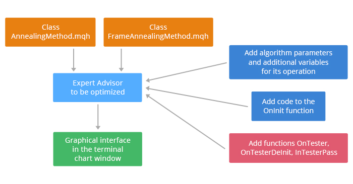
Fig. 2. Including the algorithm in the Expert Advisor
Let us now describe the AnnealingMethod and FrameAnnealingMethod classes.
The AnnealingMethod class
Here is the description of the AnnealingMethod class and more details on its methods.
#include "Math/Alglib/alglib.mqh"
//+------------------------------------------------------------------+
//|                                                                  |
//+------------------------------------------------------------------+
class AnnealingMethod
  {
private:
   CAlglib           Alg;                   // instance of the class for working with methods of the Alglib library
   CHighQualityRandStateShell state;        // instance of the class for generation of random numbers
public:
                     AnnealingMethod();
                    ~AnnealingMethod();
   struct Input                             // structure for working with the EA parameters
     {
      int               num;
      double            Value;
      double            BestValue;
      double            Start;
      double            Stop;
      double            Step;
      double            Temp;
     };
   uint              RunOptimization(string &InputParams[],int count,double F0,double T);
   uint              WriteData(Input &InpMass[],double F,int it);
   uint              ReadData(Input &Mass[],double &F,int &it);
   bool              GetParams(int Method,Input &Mass[]);
   double            FindValue(double val,double step);
   double            GetFunction(int Criterion);
   bool              Probability(double E,double T);
   double            GetT(int Method,double T0,double Tlast,int it,double D,double p1,double p2);
   double            UniformValue(double min,double max,double step);
   bool              VerificationOfVal(double start,double end,double val);
   double            Distance(double a,double b);
  };
Functions from the ALGLIB library intended for working with the random variables are used in operation of the AnnealingMethod class methods. This library is a part of the standard MetaTrader 5 package and is located in the "Include/Math/Alglib" folder, as shown below:

Fig. 3. ALGLIB library
The Private block contains declarations of the CAlglib and CHighQualityRandStateShell class instances for working with the ALGLIB functions.
To work with the optimized parameters of the EA, the Input structure has been created, which stores:
- parameter number, num;
- current value of the parameter, Value;
- the best value of the parameter, BestValue;
- initial value, Start;
- final value, Stop;
- step for changing the parameter value, Step;
- current temperature for the given parameter, Temp.
Let us consider the methods of the AnnealingMethod.mqh class.
The RunOptimization method
Designed to initialize the simulated annealing algorithm. Code of the method:
uint AnnealingMethod::RunOptimization(string &InputParams[],int count,double F0,double T)
  {
   Input Mass[];
   ResetLastError();
   bool Enable=false;
   double Start= 0;
   double Stop = 0;
   double Step = 0;
   double Value= 0;
   int j=0;
   Alg.HQRndRandomize(&state);                // initialization
   for(int i=0;i<ArraySize(InputParams);i++)
     {
      if(!ParameterGetRange(InputParams[i],Enable,Value,Start,Step,Stop))
         return GetLastError();
      if(Enable)
        {
         ArrayResize(Mass,ArraySize(Mass)+1);
         Mass[j].num=i;
         Mass[j].Value=UniformValue(Start,Stop,Step);
         Mass[j].BestValue=Mass[j].Value;
         Mass[j].Start=Start;
         Mass[j].Stop=Stop;
         Mass[j].Step=Step;
         Mass[j].Temp=T*Distance(Start,Stop);
         j++;
         if(!ParameterSetRange(InputParams[i],false,Value,Start,Stop,count))
            return GetLastError();
        }
      else
         InputParams[i]="";
     }
   if(j!=0)
     {
      if(!ParameterSetRange("iteration",true,1,1,1,count))
         return GetLastError();
      else
         return WriteData(Mass,F0,1);
     }
   return 0;
  }
Input parameters of the method:
- string array containing names of all parameters of the Expert Advisor, InputParams[];
- the number of algorithm iterations, count;
- initial value of the objective function, F0;
- initial temperature, T.
The RunOptimization method works as follows:
- It searches for the EA parameters to be optimized. Such parameters should be "ticked" in the "Parameters" tab of the Strategy Tester:
- values of each found parameter are stored in the array Mass[] of Input type structures, and the parameter is excluded from optimization. The structures array Mass[] stores:
- parameter number;
- parameter value generated by the UniformValue method (considered below);
- the maximum (Start) and maximum (Stop) values of the parameter;
- step for changing the parameter value, (Step);
- initial temperature calculated by the formula: T*Distance(Start,Stop); the Distance method will be discussed below.
- after the search is complete, all parameters are disabled and the iteration parameter is activated, which determines the number of the algorithm iterations;
- values of the Mass[] array, the objective function and the iteration number are written to a binary file using the WriteData method.
The WriteData method
Designed to write the array of parameters, values of the objective function and the iteration number to a file.
Code of the WriteData method:
uint AnnealingMethod::WriteData(Input &Mass[],double F,int it)
  {
   ResetLastError();
   int file_handle=0;
   int i=0;
   do
     {
      file_handle=FileOpen("data.bin",FILE_WRITE|FILE_BIN);
      if(file_handle!=INVALID_HANDLE) break;
      else
        {
         Sleep(MathRand()%10);
         i++;
         if(i>100) break;
        }
     }
   while(file_handle==INVALID_HANDLE);
   if(file_handle!=INVALID_HANDLE)
     {
      if(FileWriteArray(file_handle,Mass)<=0)
        {FileClose(file_handle); return GetLastError();}
      if(FileWriteDouble(file_handle,F)<=0)
        {FileClose(file_handle); return GetLastError();}
      if(FileWriteInteger(file_handle,it)<=0)
        {FileClose(file_handle); return GetLastError();}
     }
   else
      return GetLastError();
   FileClose(file_handle);
   return 0;
  }
The data are written to the data.bin file using the functions FileWriteArray, FileWriteDouble and FileWriteInteger. The method implements the ability to have multiple attempts to access the data.bin file. This is done to avoid errors when accessing the file, if the file is occupied by another process.
The ReadData method
Designed to read the array of parameters, values of the objective function and the iteration number from a file. Code of the ReadData method:
uint AnnealingMethod::ReadData(Input &Mass[],double &F,int &it)
  {
   ResetLastError();
   int file_handle=0;
   int i=0;
   do
     {
      file_handle=FileOpen("data.bin",FILE_READ|FILE_BIN);
      if(file_handle!=INVALID_HANDLE) break;
      else
        {
         Sleep(MathRand()%10);
         i++;
         if(i>100) break;
        }
     }
   while(file_handle==INVALID_HANDLE);
   if(file_handle!=INVALID_HANDLE)
     {
      if(FileReadArray(file_handle,Mass)<=0)
        {FileClose(file_handle); return GetLastError();}
      F=FileReadDouble(file_handle);
      it=FileReadInteger(file_handle);
     }
   else
      return GetLastError();
   FileClose(file_handle);
   return 0;
  }
The data are read from the file using the functions FileReadArray, FileReadDouble, FileReadInteger in the same sequence as they had been written by the WriteData method.
The GetParams method
The GetParams method is designed to calculate the new values of the expert's optimized parameters to be used in the next run of the EA. Formulas for calculating the new values of the expert's optimized parameters are provided in Table 1.
Input parameters of the method:
- variant of algorithm implementation (Boltzmann annealing, Cauchy annealing or ultrafast annealing);
- array of optimized parameters of type Input;
- coefficient CoeffTmin for calculating the minimum temperature to terminate the algorithm.
Code of the GetParams method:
bool AnnealingMethod::GetParams(int Method,Input &Mass[],double CoeffTmin)
  {
   double delta=0;
   double x1=0,x2=0;
   double count=0;

   Alg.HQRndRandomize(&state);         // initialization
   switch(Method)
     {
      case(0):
        {
         for(int i=0;i<ArraySize(Mass);i++)
           {
            if(Mass[i].Temp>=CoeffTmin*Distance(Mass[i].Start,Mass[i].Stop))
              {
               do
                 {
                  if(count==100)
                    {
                     delta=Mass[i].Value;
                     count= 0;
                     break;
                    }
                  count++;
                  delta=Mass[i].Temp*Alg.HQRndNormal(&state);
                  delta=FindValue(Mass[i].BestValue+delta,Mass[i].Step);
                 }
               //  while((delta<Mass[i].Start) || (delta>Mass[i].Stop));
               while(!VerificationOfVal(Mass[i].Start,Mass[i].Stop,delta));
               Mass[i].Value=delta;
              }
           }
         break;
        }
      case(1):
        {
         for(int i=0;i<ArraySize(Mass);i++)
           {
            if(Mass[i].Temp>=CoeffTmin*Distance(Mass[i].Start,Mass[i].Stop))
              {
               do
                 {
                  if(count==100)
                    {
                     delta=Mass[i].Value;
                     count=0;
                     break;
                    }
                  count++;
                  Alg.HQRndNormal2(&state,x1,x2);
                  delta=Mass[i].Temp*x1/x2;
                  delta=FindValue(Mass[i].BestValue+delta,Mass[i].Step);
                 }
               while(!VerificationOfVal(Mass[i].Start,Mass[i].Stop,delta));
               Mass[i].Value=delta;
              }
           }
         break;
        }
      case(2):
        {
         for(int i=0;i<ArraySize(Mass);i++)
           {
            if(Mass[i].Temp>=CoeffTmin*Distance(Mass[i].Start,Mass[i].Stop))
              {
               do
                 {
                  if(count==100)
                    {
                     delta=Mass[i].Value;
                     count=0;
                     break;
                    }
                  count++;
                  x1=Alg.HQRndUniformR(&state);
                  if(x1-0.5>0)
                     delta=Mass[i].Temp*(MathPow(1+1/Mass[i].Temp,MathAbs(2*x1-1))-1)*Distance(Mass[i].Start,Mass[i].Stop);
                  else
                    {
                     if(x1==0.5)
                        delta=0;
                     else
                        delta=-Mass[i].Temp*(MathPow(1+1/Mass[i].Temp,MathAbs(2*x1-1))-1)*Distance(Mass[i].Start,Mass[i].Stop);
                    }
                  delta=FindValue(Mass[i].BestValue+delta,Mass[i].Step);
                 }
               while(!VerificationOfVal(Mass[i].Start,Mass[i].Stop,delta));
               Mass[i].Value=delta;
              }
           }
         break;
        }
      default:
        {
         Print("Annealing method was chosen incorrectly");
         return false;
        }
     }
   return true;
  }
Let us consider the code of this method in more detail.
This method has a switch operator for starting the calculation of new parameter values depending on the selected algorithm implementation variant. The new parameter values are only calculated if the current temperature is above the minimum. The minimum temperature is calculated by the formula: CoeffTmin*Distance(Start,Stop), where Start and Stop are the minimum and maximum values of the parameter. The Distance method will be considered below.
The HQRndRandomize method of the CAlglib class is called to initialize the methods for working with random numbers.
Alg.HQRndRandomize(&state);
The HQRndNormal function of the CAlglib class is used for calculating the value of the standard normal distribution:
Alg.HQRndNormal(&state);
Cauchy distributions can be modeled in various ways, for example, through normal distribution or inverse functions. The following ratio will be used:
C(0,1)=X1/X2, where X1 and X2 are normally distributed independent variables, X1,X2 = N(0,1). The HQRndNormal2 function of the CAlglib class is used to generate two normally distributed variables:
Alg.HQRndNormal2(&state,x1,x2);
Values of normally distributed independent variables are stored in x1, x2.
The HQRndUniformR(&state) method of the CAlglib class generates a random number, uniformly distributed in the interval from 0 to 1:
Alg.HQRndUniformR(&state);
Using the FindValue method (described below), the calculated parameter value is rounded to the specified step for changing the parameter. If the calculated parameter value exceeds the parameter changing range (checked by the VerificationOfVal method), it is recalculated.
The FindValue method
The value of each optimized parameter should be changed with the specified step. A new value generated in GetParams may not meet this condition, and it will need to be rounded to a multiple of the specified step. This is done by the FindValue method. Input parameters of the method: the value to be rounded (val), and the step for changing the parameter (step).
Here is the code of the FindValue method:
double AnnealingMethod::FindValue(double val,double step)
  {
   double buf=0;
   if(val==step)
      return val;
   if(step==1)
      return round(val);
   else
     {

      buf=(MathAbs(val)-MathMod(MathAbs(val),MathAbs(step)))/MathAbs(step);
      if(MathAbs(val)-buf*MathAbs(step)>=MathAbs(step)/2)
        {
         if(val<0)
            return -(buf + 1)*MathAbs(step);
         else
            return (buf + 1)*MathAbs(step);
        }
      else
        {
         if(val<0)
            return -buf*MathAbs(step);
         else
            return buf*MathAbs(step);
        }
     }
  }
Let us consider the code of this method in more detail.
If the step is equal to the input value of the parameter, the function returns that value:
   if(val==step)
      return val;
If the step is 1, the input value of the parameter only needs to be rounded to the integer:
   if(step==1)
      return round(val);
Otherwise, find the number of steps in the input value of the parameter:
buf=(MathAbs(val)-MathMod(MathAbs(val),MathAbs(step)))/MathAbs(step);
and calculate a new value, which is a multiple of the step.
The GetFunction method
The GetFunction method is designed to obtain the new value of the objective function. The input parameter of the method is the user-defined optimization criterion.
Depending on the selected calculation mode, the objective function takes the value of one or several statistic parameters calculated from the test results. Code of the method:
double AnnealingMethod::GetFunction(int Criterion)
  {
   double Fc=0;
   switch(Criterion)
     {
      case(0):
         return TesterStatistics(STAT_PROFIT);
      case(1):
         return TesterStatistics(STAT_PROFIT_FACTOR);
      case(2):
         return TesterStatistics(STAT_RECOVERY_FACTOR);
      case(3):
         return TesterStatistics(STAT_SHARPE_RATIO);
      case(4):
         return TesterStatistics(STAT_EXPECTED_PAYOFF);
      case(5):
         return TesterStatistics(STAT_EQUITY_DD);//min
      case(6):
         return TesterStatistics(STAT_BALANCE_DD);//min
      case(7):
         return TesterStatistics(STAT_PROFIT)*TesterStatistics(STAT_PROFIT_FACTOR);
      case(8):
         return TesterStatistics(STAT_PROFIT)*TesterStatistics(STAT_RECOVERY_FACTOR);
      case(9):
         return TesterStatistics(STAT_PROFIT)*TesterStatistics(STAT_SHARPE_RATIO);
      case(10):
         return TesterStatistics(STAT_PROFIT)*TesterStatistics(STAT_EXPECTED_PAYOFF);
      case(11):
        {
         if(TesterStatistics(STAT_BALANCE_DD)>0)
            return TesterStatistics(STAT_PROFIT)/TesterStatistics(STAT_BALANCE_DD);
         else
            return TesterStatistics(STAT_PROFIT);
        }
      case(12):
        {
         if(TesterStatistics(STAT_EQUITY_DD)>0)
            return TesterStatistics(STAT_PROFIT)/TesterStatistics(STAT_EQUITY_DD);
         else
            return TesterStatistics(STAT_PROFIT);
        }
      case(13):
        {
         // specify the custom criterion, for example
         return TesterStatistics(STAT_TRADES)*TesterStatistics(STAT_PROFIT);
        }
      default: return -10000;
     }
  }
As you can see from the code, 14 ways to calculate the objective function are implemented in the method. That is, users can optimize an expert by various statistic parameters. The detailed description of the statistic parameters is available in the documentation.
The Probability method
The Probability method is designed to identify a transition to a new state. Input parameters of the method: difference between the previous and current values of the objective function (E) and the current temperature (T). Code of the method:
bool AnnealingMethod::Probability(double E,double T)
  {
   double a=Alg.HQRndUniformR(&state);
   double res=exp(-E/T);
   if(res<=a)
      return false;
   else
      return true;
  }
The method generates a random variable а, uniformly distributed over the interval from 0 to 1:
a=Alg.HQRndUniformR(&state);
The obtained value is compared with the expression exp(-E/T). If a>exp(-E/T), then the method returns true (transition to a new state is performed).
The GetT method
The GetT method calculates the new temperature value. Input parameters of the method:
- variant of algorithm implementation (Boltzmann annealing, Cauchy annealing or ultrafast annealing);
- initial value of temperature, T0;
- previous value of temperature, Tlast;
- iteration number, it;
- the number of optimized parameters, D;
- auxiliary parameters p1 and p2 for the ultrafast annealing.
Code of the method:
double AnnealingMethod::GetT(int Method,double T0,double Tlast,int it,double D,double p1,double p2)
  {
   int Iteration=0;
   double T=0;
   switch(Method)
     {
      case(0):
        {
         if(Tlast!=T0)
            Iteration=(int)MathRound(exp(T0/Tlast)-1)+1;
         else
            Iteration=1;
         if(Iteration>0)
            T=T0/log(Iteration+1);
         else
            T=T0;
         break;
        }
      case(1):
        {
         if(it!=1)
            Iteration=(int)MathRound(pow(T0/Tlast,D))+1;
         else
            Iteration=1;
         if(Iteration>0)
            T=T0/pow(Iteration,1/D);
         else
            T=T0;
         break;
        }
      case(2):
        {
         if((T0!=Tlast) && (-p1*exp(-p2/D)!=0))
            Iteration=(int)MathRound(pow(log(Tlast/T0)/(-p1*exp(-p2/D)),D))+1;
         else
            Iteration=1;
         if(Iteration>0)
            T=T0*exp(-p1*exp(-p2/D)*pow(Iteration,1/D));
         else
            T=T0;
         break;
        }
     }
   return T;
  }
The method calculates the new temperature value depending on the variant of the algorithm implementation according to the formulas in Table 2. In order to take into account the algorithm implementation that increases the temperature only when a transition to a new state occurs, the current iteration is calculated using the previous temperature value Tlast. Thus, the current temperature is decreased when the method is called, regardless of the current iteration of the algorithm.
The UniformValue method
The UniformValue method generates a random value of the optimized parameter, considering its minimum, maximum values and step. The method is used only during the initialization of the algorithm, to generate the initial values of the optimized parameters. Input parameters of the method:
- the maximum parameter value, max;
- the minimum parameter value, min;
- step for changing the parameter, step.
Code of the method:
double AnnealingMethod::UniformValue(double min,double max,double step)
  {
   Alg.HQRndRandomize(&state);       //initialization
   if(max>min)
      return FindValue(Alg.HQRndUniformR(&state)*(max-min)+min,step);
   else
      return FindValue(Alg.HQRndUniformR(&state)*(min-max)+max,step);
  }
The VerificationOfVal method
The VerificationOfVal checks if the specified value of the (val) variable is out of range (start,end). This method is used in the GetParams method.
Code of the method:
bool AnnealingMethod::VerificationOfVal(double start,double end,double val)
  {
   if(start<end)
     {
      if((val>=start) && (val<=end))
         return true;
      else
         return false;
     }
   else
     {
      if((val>=end) && (val<=start))
         return true;
      else
         return false;
     }
  }
The method takes into account that the parameter changing step may be negative, therefore, it checks the condition "start<end".
The Distance method
The Distance method calculates the distance between two parameters (a and b) and is used in the algorithm for calculating the parameter change range with the initial value of a and the final value of b.
Code of the method:
double AnnealingMethod::Distance(double a,double b)
  {
   if(a<b)
      return MathAbs(b-a);
   else
      return MathAbs(a-b);
  }
The FrameAnnealingMethod class
The FrameAnnealingMethod class is designed to display the algorithm execution process in the terminal window. Here is the description of the FrameAnnealingMethod class:
#include <SimpleTable.mqh>
#include <Controls\BmpButton.mqh>
#include <Controls\Label.mqh>
#include <Controls\Edit.mqh>
#include <AnnealingMethod.mqh>
//+------------------------------------------------------------------+
//| Class for the output of the optimization results                 |
//+------------------------------------------------------------------+
class FrameAnnealingMethod
  {
private:
   CSimpleTable      t_value;
   CSimpleTable      t_inputs;
   CSimpleTable      t_stat;
   CBmpButton        b_playbutton;
   CBmpButton        b_backbutton;
   CBmpButton        b_forwardbutton;
   CBmpButton        b_stopbutton;
   CLabel            l_speed;
   CLabel            l_stat;
   CLabel            l_value;
   CLabel            l_opt_value;
   CLabel            l_temp;
   CLabel            l_text;
   CLabel            n_frame;
   CEdit             e_speed;
   long              frame_counter;

public:
   //--- constructor/destructor
                     FrameAnnealingMethod();
                    ~FrameAnnealingMethod();
   //--- Events of the strategy tester
   void              FrameTester(double F,double Fbest,Input &Mass[],int num,int it);
   void              FrameInit(string &SMass[]);
   void              FrameTesterPass(int cr);
   void              FrameDeinit(void);
   void              FrameOnChartEvent(const int id,const long &lparam,const double &dparam,const string &sparam,int cr);
   uint              FrameToFile(int count);
  };
The FrameAnnealingMethod class contains the following methods:
- FrameInit — create a graphical interface in the terminal window;
- FrameTester — add the current data frame;
- FrameTesterPass — output the current data frame to the terminal window;
- FrameDeInit — display the text information about the completion of the expert optimization;
- FrameOnChartEvent — handle the button press events;
- FrameToFile — save the testing results to a text file.
The code of the methods is provided in the FrameAnnealingMethod.mqh file (attached to the article). Please note that the SimpleTable.mqh file (attached to the article) is required for the methods in the FrameAnnealingMethod class to work. Place it in MQL5/Include. The file has been adopted from this project and is supplemented with the GetValue method, which allows reading a value from a table cell.
Here is a sample graphical interface created in the terminal window using the FrameAnnealingMethod class.
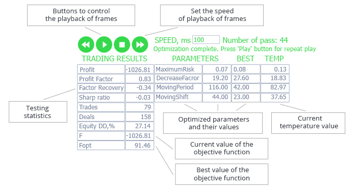
Fig. 4. Graphical interface for demonstrating the operation of the algorithm
The left side of the table contains statistic parameters generated by the strategy tester based on the results of the current run, as well as the current and the best values of the objective function (in this example, the net profit is chosen as the objective function).
Optimized parameters are located in the right side of the table: parameter name, current value, best value, current temperature.
Above the table, there are buttons to control the playback of frames after the algorithm execution is complete. Thus, after an expert optimization is complete, you can replay it at the specified speed. The buttons allow you to stop the playback of frames and start it again from the frame, where the playback was interrupted. The playback speed can be adjusted using the buttons, or it can be set manually. The number of the current run is displayed to the right of the speed value. Auxiliary information on the algorithm operation is displayed below.
The AnnealingMethod and FrameAnnealingMethod classes have been considered. Now let us proceed to testing the algorithm using an Expert Advisor based on Moving Average as an example.
Testing the algorithm on the EA based on Moving Average
Preparing the EA for testing the algorithm
The expert's code should be modified to run the algorithm:
- include the classes AnnealingMethod and FrameAnnealingMethod, and declare auxiliary variables for the operation of the algorithm;
- add the code to the OnInit function, add the functions OnTester, OnTesterInit, OnTesterDeInit, OnTesterPass, OnChartEvent.
The added code does not affect the EA operation and is only run when the EA is optimized in the strategy tester.
So, let us begin.
Include the file with the initial parameters, generated by the OnTesterInit function:
#property tester_file "data.bin"
Include the classes AnnealingMethod and FrameAnnealingMethod:
// including classes
#include <AnnealingMethod.mqh>
#include <FrameAnnealingMethod.mqh>
Declare instances of the included classes:
AnnealingMethod Optim;
FrameAnnealingMethod Frame;
Declare the auxiliary variables for the operation of the algorithm:
Input InputMass[];            // array of input parameters
string SParams[];             // array of input parameter names
double Fopt=0;                // the best value of the function
int it_agent=0;               // algorithm iteration number for the testing agent
uint alg_err=0;               // error number
The simulated annealing algorithm will modify the values of the optimized parameters over the course of its work. For this purpose, the input parameters of the EA will be renamed:
double MaximumRisk_Optim=MaximumRisk;
double DecreaseFactor_Optim=DecreaseFactor;
int MovingPeriod_Optim=MovingPeriod;
int MovingShift_Optim=MovingShift;
In all functions of the EA, replace the parameters: MaximumRisk with MaximumRisk_Optim, DecreaseFactor with DecreaseFactor_Optim, MovingPeriod with MovingPeriod_Optim, MovingShift with MovingShift_Optim.
Here are the variables for configuring the operation of the algorithm:
sinput int iteration=50;         // Number of iterations
sinput int method=0;             // 0 - Boltzmann annealing, 1 - Cauchy annealing, 2 - ultrafast annealing
sinput double CoeffOfTemp=1;     // Scale coefficient for the initial temperature
sinput double CoeffOfMinTemp=0;  // Coefficient for the minimum temperature
sinput double Func0=-10000;      // Initial value of the objective function
sinput double P1=1;              // Additional parameter for the ultrafast annealing, p1
sinput double P2=1;              // Additional parameter for the ultrafast annealing, p2
sinput int Crit=0;               // Objective function calculation method
sinput int ModOfAlg=0;           // Algorithm modification type
sinput bool ManyPoint=false;     // Multiple point optimization
Parameters of the algorithm should not change during its operation; therefore, all variables are declared with the sinput identifier.
Table 3 explains the purpose of the declared variables.
Table 3
| Variable name | Purpose |
|---|---|
| iteration | Defines the number of algorithm iterations |
| method | Defines the variant of algorithm implementation: 0 — Boltzmann annealing, 1 — Cauchy annealing, 2 — ultrafast annealing |
| CoeffOfTemp | Defines the coefficient for setting the initial temperature calculated by the formula: T0=CoeffOfTemp*Distance(Start,Stop), where Start, Stop are the minimum and maximum values of the parameter, Distance is a method of the AnnealingMethod class (described above) |
| CoeffOfMinTemp | Defines the coefficient for setting the minimum temperature to terminate the algorithm. The maximum temperature is calculated similarly to the initial temperature: Tmin=CoeffOfMinTemp*Distance(Start,Stop), where Start, Stop the minimum and maximum values of the parameter, Distance is a method of the AnnealingMethod class (described above) |
| Func0 | Initial value of the objective function |
| P1,P2 | Parameters used for calculation of the current temperature in ultrafast annealing (see Table 2) |
| Crit | Optimization criterion: 0 — Total Net Profit; 1 — Profit Factor; 2 — Recovery Factor; 3 — Sharpe Ratio; 4 — Expected Payoff; 5 — Equity Drawdown Maximal; 6 — Balance Drawdown Maximal; 7 — Total Net Profit + Profit Factor; 8 — Total Net Profit + Recovery Factor; 9 — Total Net Profit + Sharpe Ratio; 10 — Total Net Profit + Expected Payoff; 11 — Total Net Profit + Balance Drawdown Maximal; 12 — Total Net Profit + Equity Drawdown Maximal; 13 — Custom criterion. The objective function is calculated in the GetFunction function of the AnnealingMethod class |
| ModOfAlg | Type of algorithm modification: 0 - if a transition to a new state has occurred, decrease the current temperature and proceed to the check of algorithm completion, otherwise, calculate the new values of the optimized parameters; 1 - regardless of the result of checking the transition to a new state, decrease the current temperature and proceed to the check of algorithm completion |
| ManyPoint | true — different initial values of the optimized parameters will be generated for each testing agent, false — the same initial values of the optimized parameters will be generated for each testing agent |
Add the code to the beginning of the OnInit function:
//+------------------------------------------------------------------+
//| Simulated annealing                                              |
//+------------------------------------------------------------------+
 if(MQL5InfoInteger(MQL5_OPTIMIZATION))
    {
     // open the file and read data
     //  if(FileGetInteger("data.bin",FILE_EXISTS,false))
     //  {
         alg_err=Optim.ReadData(InputMass,Fopt,it_agent);
         if(alg_err==0)
           {
            // If it is the first run, generate the parameters randomly, if the search is performed from different points
            if(Fopt==Func0)
              {
               if(ManyPoint)
                  for(int i=0;i<ArraySize(InputMass);i++)
                    {
                     InputMass[i].Value=Optim.UniformValue(InputMass[i].Start,InputMass[i].Stop,InputMass[i].Step);
                     InputMass[i].BestValue=InputMass[i].Value;
                    }
              }
            else
               Optim.GetParams(method,InputMass,CoeffOfMinTemp);    // generate new parameters
            // fill the parameters of the Expert Advisor
            for(int i=0;i<ArraySize(InputMass);i++)
               switch(InputMass[i].num)
                 {
                  case (0): {MaximumRisk_Optim=InputMass[i].Value; break;}
                  case (1): {DecreaseFactor_Optim=InputMass[i].Value; break;}
                  case (2): {MovingPeriod_Optim=(int)InputMass[i].Value; break;}
                  case (3): {MovingShift_Optim=(int)InputMass[i].Value; break;}
                 }
           }
         else
           {
            Print("Error reading file");
            return(INIT_FAILED);
           }
//+------------------------------------------------------------------+
//|                                                                  |
//+------------------------------------------------------------------+
Let's examine the code in details. The added code is executed only in the optimization mode of the strategy tester:
if(MQL5InfoInteger(MQL5_OPTIMIZATION))
Next, the data are read from the data.bin file, generated by the RunOptimization method of the AnnealingMethod class. This method is called in the OnTesterInit function, the function code will be shown below.
alg_err=Optim.ReadData(InputMass,Fopt,it_agent);
If the data were read without errors (alg_err=0), a check is performed to see if algorithm is at the first iteration (Fopt==Func0), otherwise the EA initialization fails with an error. If it is the first iteration, and if ManyPoint = true, the initial values of the optimized parameters are generated and stored in the InputMass structure of the Input type (described in the AnnealingMethod class), otherwise the GetParams method is called
Optim.GetParams(method,InputMass,CoeffOfMinTemp);// generate new parameters
and the values of parameters MaximumRisk_Optim, DecreaseFactor_Optim, MovingPeriod_Optim, MovingShift_Optim are filled.
Now let us consider the code of the OnTesterInit function:
void OnTesterInit()
  {
  // fill the array of names of all EA parameters
   ArrayResize(SParams,4);
   SParams[0]="MaximumRisk";
   SParams[1]="DecreaseFactor";
   SParams[2]="MovingPeriod";
   SParams[3]="MovingShift";
   // start the optimization
   Optim.RunOptimization(SParams,iteration,Func0,CoeffOfTemp);
   // create the graphical interface
   Frame.FrameInit(SParams);
  }
First, fill the string array that contains the names of all EA parameters. Then run the RunOptimization method and create a graphical interface using the FrameInit method.
After running the EA on the specified time interval, the control will be transferred to the OnTester function. Here is its code:
double OnTester()
  {
   int i=0;                                                       // cycle counter
   int count=0;                                                   // auxiliary variable
  // check for completion of the algorithm when the minimum temperature is reached
   for(i=0;i<ArraySize(InputMass);i++)
      if(InputMass[i].Temp<CoeffOfMinTemp*Optim.Distance(InputMass[i].Start,InputMass[i].Stop))
         count++;
   if(count==ArraySize(InputMass))
      Frame.FrameTester(0,0,InputMass,-1,it_agent);               // add a new frame with zero parameters and id=-1
   else
     {
      double Fnew=Optim.GetFunction(Crit);                        // calculate the current value of the function
      if((Crit!=5) && (Crit!=6) && (Crit!=11) && (Crit!=12))      // if it is necessary to maximize the objective function
        {
         if(Fnew>Fopt)
            Fopt=Fnew;
         else
           {
            if(Optim.Probability(Fopt-Fnew,CoeffOfTemp*InputMass[0].Temp/Optim.Distance(InputMass[0].Start,InputMass[0].Stop)))
               Fopt=Fnew;
           }
        }
      else                                                        // if it is necessary to minimize the objective function
        {
         if(Fnew<Fopt)
            Fopt=Fnew;
         else
           {
            if(Optim.Probability(Fnew-Fopt,CoeffOfTemp*InputMass[0].Temp/Optim.Distance(InputMass[0].Start,InputMass[0].Stop)))
               Fopt=Fnew;
           }
        }
      // overwrite the best parameters values
      if(Fopt==Fnew)
         for(i=0;i<ArraySize(InputMass);i++)
            InputMass[i].BestValue=InputMass[i].Value;
      // decrease the temperature
      if(((ModOfAlg==0) && (Fnew==Fopt)) || (ModOfAlg==1))
        {
         for(i=0;i<ArraySize(InputMass);i++)
            InputMass[i].Temp=Optim.GetT(method,CoeffOfTemp*Optim.Distance(InputMass[i].Start,InputMass[i].Stop),InputMass[i].Temp,it_agent,ArraySize(InputMass),P1,P2);
        }
      Frame.FrameTester(Fnew,Fopt,InputMass,iteration,it_agent);          // add a new frame
      it_agent++;                                                         // increase the iteration counter
      alg_err=Optim.WriteData(InputMass,Fopt,it_agent);                   // write the new values to the file
      if(alg_err!=0)
         return alg_err;
     }
   return Fopt;
  }
Let us consider the code of this function in more detail.
- It checks for completion of the algorithm when the minimum temperature is reached. If the temperature of each parameter has reached the minimum value, a frame with id=-1 is added, the parameter values do not change anymore. The graphical interface in the terminal window prompts the user to complete the optimization by pressing the "Stop" button in the strategy tester.
- The GetFunction method calculates the new value of the objective function Fnew, using the Expert Advisor test results.
- Depending on the optimization criterion (see Table 3), the value of Fnew is compared with the best value of Fopt, and the transition to a new state is checked.
- If a transition to a new state has occurred, the current values of the optimized parameters are set as the best:
 for(i=0;i<ArraySize(InputMass);i++)
         InputMass[i].BestValue = InputMass[i].Value;
- The condition for decreasing the current temperature is checked. If it is met, the new temperature is calculated using the GetT method of the AnnealingMethod class.
- A new frame is added, the values of the optimized parameters are written to the file.
The OnTester function adds frames to be further processed in the OnTesterPass function. Here is its code:
void OnTesterPass()
  {
      Frame.FrameTesterPass(Crit);// method to display the frames in the graphical interface
  }
The OnTesterPass function calls the FrameTesterPass method of the FrameAnnealingMethod class to display the optimization process in the terminal window.
Once the optimization is complete, the OnTesterDeInit function is called:
void OnTesterDeinit()
  {
   Frame.FrameToFile(4);
   Frame.FrameDeinit();
  }
This function calls two methods of the FrameAnnealingMethod class: FrameToFile and FrameDeinit. The FrameToFile method writes the optimization results to a text file. This method takes the number of the EA's parameters to be optimized as input. The FrameDeinit method outputs a message about the optimization completion to the terminal window.
Once the optimization is complete, the graphical interface created using the FrameAnnealingMethod class methods allows playing the frames at a specified speed. The playback of frames can be stopped and restarted. This is done by the corresponding buttons of the graphical interface (see Fig. 4). To handle the events in the terminal window, the OnChartEvent method has been added to the EA code:
void OnChartEvent(const int id,const long &lparam,const double &dparam,const string &sparam)
  {
   Frame.FrameOnChartEvent(id,lparam,dparam,sparam,Crit); // method for working with the graphical interface
  }
The OnChartEvent method calls the FrameOnChartEvent method of the FrameAnnealingMethod class, which manages the playback of frames in the terminal window.
This concludes the modification of the MovingAverage EA code. Let us start testing the algorithm.
Testing the algorithm
The proposed simulated annealing method has a stochastic nature (it contains functions for calculating random variables), therefore, each run of the algorithm will produce a different result. To test the algorithm operation and to identify its advantages and disadvantages, it is necessary to run the expert optimization many times. This would take a considerable amount of time, so the following will be done: run optimization in the "Slow complete algorithm" mode, save the obtained results and then test the algorithm using these data.
The algorithm will be tested using the TestAnnealing.mq5 Expert Advisor (located in the test.zip file attached to the article). It loads a table of optimization results obtained by the full search method from a text file containing 5 columns with data: columns 1-4 represent the values of variables, column 5 shows the values of the objective function. The algorithm implemented in TestAnnealing uses the simulated annealing method to move through the table and find the values of the objective function. This testing approach allows checking the performance of simulated annealing on various data obtained by the complete search.
So, let us start. First, test the algorithm performance by optimizing one variable of the expert — Moving Average period.
Run the expert optimization in the complete search mode with the following initial parameters:
- Maximum Risk in percentage — 0.02; Decrease factor — 3; Moving Average period: 1 - 120, step: 1; Moving Average shift — 6.
- Period: 01.01.2017 — 31.12.2017, trading mode: no delay, ticks: 1 minute OHLC, initial deposit: 10000, leverage: 1:100, currency: EURUSD.
- Optimization will be performed using the criterion Balance max.
Save the result and create a test file with the obtained data. The data in the text file will be sorted in ascending order of the "Moving Average period" parameter value, as shown in Fig. 5.
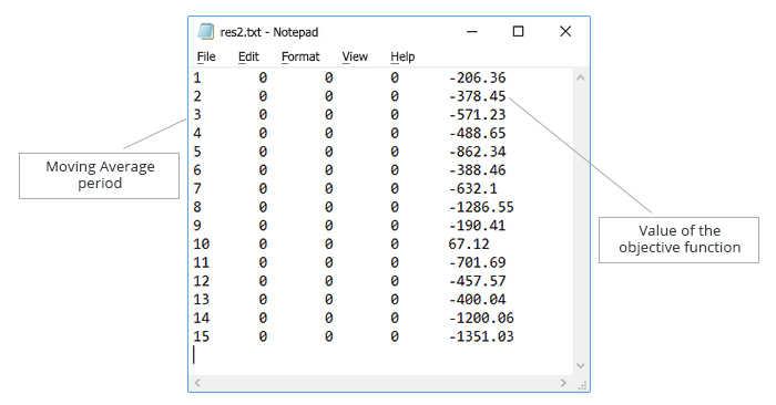
Fig. 5. Optimization of the "Moving Average period" parameter. Text file with the data for testing the algorithm operation
120 iterations were performed in the complete search mode. The algorithm of simulated annealing will be tested with the following number of iterations: 30 (variant 1), 60 (variant 2), 90 (variant 3). The purpose here is to test the performance of the algorithm while reducing the number of iterations.
For each variant, 10000 optimization runs using simulated annealing were performed on the data obtained by the complete search. The algorithm implemented in the TestAnnealing.mq5 Expert Advisor counts how many times the best value of the objective function was found, as well as how many times the objective function values differing from the best one by 5%, 10%, 15%, 20%, 25% were found.
The following test results have been obtained.
For 30 iterations of the algorithm, the best values were obtained by the ultrafast annealing with temperature reduction on each iteration:
| Deviation from the best value of the objective function, % | Result, % |
|---|---|
| 0 | 33 |
| 5 | 44 |
| 10 | 61 |
| 15 | 61 |
| 20 | 72 |
| 25 | 86 |
The data of this table are interpreted as: the best value of the objective function was obtained in 33% of the runs (in 3,300 out of 10,000 runs), 5% deviation from the best value was obtained in 44% of the runs, and so on.
For 60 iterations of the algorithm, Cauchy annealing is leading, but the best variant here was the temperature reduction during the transition to a new state. The results are as follows:
| Deviation from the best value of the objective function, % | Result, % |
|---|---|
| 0 | 47 |
| 5 | 61 |
| 10 | 83 |
| 15 | 83 |
| 20 | 87 |
| 25 | 96 |
Thus, with the iteration count halved compared to the complete search, the simulated annealing method finds the best value of the objective function in 47% of the cases.
For 90 iterations or the algorithm, Boltzmann annealing and Cauchy annealing with temperature reduction during the transition to a new state had approximately the same result. Here are the results for the Cauchy annealing:
| Deviation from the best value of the objective function, % | Result, % |
|---|---|
| 0 | 62 |
| 5 | 71 |
| 10 | 93 |
| 15 | 93 |
| 20 | 95 |
| 25 | 99 |
Thus, with the iteration count decreased by a third compared to the complete search, the simulated annealing method finds the best value of the objective function in 62% of the cases. However, it is possible to obtain quite acceptable results with a deviation of 10-15%.
The ultrafast annealing method was tested with parameters p1=1, p2=1. Increasing the number of iterations had a greater negative impact on the obtained result than on that of Boltzmann annealing and Cauchy annealing. However, the ultrafast annealing algorithm has one peculiarity: changing the coefficients p1, p2 allows adjusting the temperature reduction speed.
Let us consider the temperature change graph for ultrafast annealing (Fig. 6):


Fig. 6. The temperature change graph for ultrafast annealing (T0=100, n=4)
Fig. 6 implies that it is necessary to increase the coefficient p1 and decrease the coefficient p2 in order to reduce the rate of temperature change. Accordingly, to increase the rate of temperature change, it is necessary to reduce the coefficient p1 and increase the coefficient p2.
At 60 and 90 iterations, ultrafast annealing showed the worst results because the temperature was falling too fast. After decreasing the coefficient p1, the following results were obtained:
| Number of iterations | p1 | p2 | 0% | 5% | 10% | 15% | 20% | 25% |
|---|---|---|---|---|---|---|---|---|
| 60 | 0.5 | 1 | 57 | 65 | 85 | 85 | 91 | 98 |
| 90 | 0.25 | 1 | 63 | 78 | 93 | 93 | 96 | 99 |
The table shows that the best value of the objective function was obtained in 57% of the runs at 60 iterations and in 63% of the runs at 90 iterations.
Thus, the best result when optimizing one parameter was achieved by the ultrafast annealing. However, it is necessary to select the coefficients p1 and p2 depending on the number of iterations.
As mentioned above, the simulated annealing algorithm is stochastic, so its operation will be compared with random search. To do this, a random value of a parameter with a given step and in a given range will be generated at each iteration. In this case, the values of the "Moving Average period" parameter will be generated with a step of 1, in the range from 1 to 120.
The random search was performed with the same conditions as the simulated annealing:
- number of iterations: 30, 60, 90
- number of runs in each variant: 10000
The results of the random search are presented in the table below:
| Number of iterations | 0% | 5% | 10% | 15% | 20% | 25% |
|---|---|---|---|---|---|---|
| 30 | 22 | 40 | 54 | 54 | 64 | 84 |
| 60 | 40 | 64 | 78 | 78 | 87 | 97 |
| 90 | 52 | 78 | 90 | 90 | 95 | 99 |
Let us compare the results of random search and ultrafast annealing. The table shows the percentage increase between the corresponding values of random search and ultrafast annealing. For instance, at 30 iterations, the ultrafast annealing algorithm is 50% better at finding the best value of the function than random search.
| Number of iterations | 0% | 5% | 10% | 15% | 20% | 25% |
|---|---|---|---|---|---|---|
| 30 | 50 | 10 | 12.963 | 12.963 | 12.5 | 2.381 |
| 60 | 42.5 | 1.563 | 8.974 | 8.974 | 4.6 | 1.031 |
| 90 | 21.154 | 0 | 3.333 | 3.333 | 1.053 | 0 |
The table shows that increasing the number of iterations reduces the advantage of the ultrafast annealing algorithm.
Now let us proceed to testing the algorithm on optimization of two parameters of the Expert Advisor, "Moving Average period" and "Moving Average shift". First, generate the input data by running the slow complete search in the strategy tester with the following parameters:
- Maximum Risk in percentage — 0.02; Decrease factor — 3; Moving Average period: 1-120; Moving Average shift - 6-60.
- Period: 01.01.2017 — 31.12.2017, trading mode: no delay, ticks: 1 minute OHLC, initial deposit: 10000, leverage: 1:100, currency: EURUSD
- Optimization will be performed using the criterion Balance max.
Save the result and create a test file with the obtained data. The data in the text file are sorted in the ascending order of the "Moving Average period" parameter. The generated file is shown in Fig. 7.
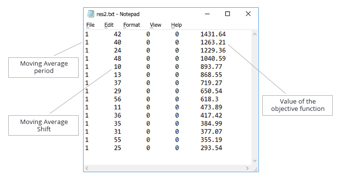
Fig. 7. Optimization of the "Moving Average period" and "Moving Average shift" parameters. Text file with the data for testing the algorithm operation
The slow complete search for two variables is performed in 6,600 iterations. We will try to reduce this number using simulated annealing. Test the algorithm with the following number of iterations: 330, 660, 1665, 3300, 4950. The number of runs in each variant: 10000.
The testing results are as follows.
330 iterations: Cauchy annealing showed good results, but the best result was achieved by ultrafast annealing with temperature reduction on each iteration and coefficients p1=1, p2=1.
660 iterations: results of Cauchy annealing ultrafast annealing with temperature reduction on each iteration and coefficients p1=1, p2=1 showed approximately the same results.
At 1665, 3300 and 4950 iterations, the best result was achieved by ultrafast annealing with temperature reduction on each iteration and the following values of the p1 and p2 coefficients:
- 1665 iterations: p1= 0.5, p2=1
- 3300 iterations: p1= 0.25, p2=1
- 4950 iterations: p1= 0.5, p2=3
The best results are summarized in the table:
| Number of iterations | 0% | 5% | 10% | 15% | 20% | 25% |
|---|---|---|---|---|---|---|
| 330 | 11 | 11 | 18 | 40 | 66 | 71 |
| 660 | 17 | 17 | 27 | 54 | 83 | 88 |
| 1665 | 31 | 31 | 41 | 80 | 95 | 98 |
| 3300 | 51 | 51 | 62 | 92 | 99 | 99 |
| 4950 | 65 | 65 | 75 | 97 | 99 | 100 |
The following conclusions can be drawn from the table:
- when the number of iterations is reduced by 10 times, the ultrafast annealing algorithm finds the best value of the objective function in 11% of the cases; but in 71% of the cases, it produces a value of the objective function that is only 25% worse than the best one.
- when the number of iterations is reduced by 2 times, the ultrafast annealing algorithm finds the best value of the objective function in 51% of the cases; but it has almost 100% probability to find a value of the objective function that is only 20% worse than the best one.
Thus, the ultrafast annealing algorithm can be used to quickly assess the profitability of strategies when a small deviation from the best value is perfectly acceptable.
Now let us compare the ultrafast annealing algorithm with random search. The results of the random search are presented in the table below:
| Number of iterations | 0% | 5% | 10% | 15% | 20% | 25% |
|---|---|---|---|---|---|---|
| 330 | 5 | 5 | 10 | 14 | 33 | 42 |
| 660 | 10 | 10 | 19 | 27 | 55 | 67 |
| 1665 | 22 | 22 | 41 | 53 | 87 | 94 |
| 3300 | 40 | 40 | 64 | 79 | 98 | 99 |
| 4950 | 55 | 55 | 79 | 90 | 99 | 99 |
Let us compare the results of random search and ultrafast annealing. The results will be represented in the form of a table that shows the percentage increase between the corresponding values of random search and ultrafast annealing.
| Number of iterations | 0% | 5% | 10% | 15% | 20% | 25% |
|---|---|---|---|---|---|---|
| 330 | 120 | 120 | 80 | 185.714 | 100 | 69 |
| 660 | 70 | 70 | 42.105 | 100 | 50.909 | 31.343 |
| 1665 | 40.909 | 40.909 | 0 | 50.9434 | 9.195 | 4.255 |
| 3300 | 27.5 | 27.5 | -3.125 | 16.456 | 1.021 | 0 |
| 4950 | 18.182 | 18.182 | -5.064 | 7.778 | 0 | 1.01 |
Thus, a significant advantage of the ultrafast annealing algorithm is observed on a small number of iterations. When it increases, the advantage decreases and sometimes even becomes negative. Note that a similar situation took place when testing the algorithm by optimizing one parameter.
Now, to the main point: compare the ultrafast annealing algorithm and genetic algorithm (GA), integrated into the strategy tester.
Comparison of GA and ultrafast annealing in optimization of two variables: "Moving Average period" and "Moving Average shift"
The algorithms will start with the following initial parameters:
- Maximum Risk in percentage — 0.02; Decrease factor — 3; Moving Average period: 1 — 120, step: 1; Moving Average shift — 6-60, step: 1
- Period: 01.01.2017 — 31.12.2017, trading mode: no delay, ticks: 1 minute OHLC, initial deposit: 10000, leverage: 1:100, currency: EURUSD
- Optimization will be performed using the criterion Balance max
Run the genetic algorithm 20 times, save the results and the average number of iterations needed to complete the algorithm.
After 20 runs of GA, the following values were obtained: 1392.29; 1481.32; 2284.46; 1665.44; 1435.16; 1786.78; 1431.64; 1782.34; 1520.58; 1229.36; 1482.23; 1441.36; 1763.11; 2286.46; 1476.54; 1263.21; 1491.09; 1076.9; 913.42; 1391.72.
Average number of iterations: 175; average value of the objective function: 1529.771.
Given that the best value of the objective function is 2446.33, GA does not produce a good result, with the average value of the objective function being only 62.53% of the best value.
Now perform 20 runs of the ultrafast annealing algorithm at 175 iterations with the parameters: p1=1, p2=1.
The ultrafast annealing was launched on 4 testing agents, while the search for the objective function was performed autonomously on each agent, so that each agent performed 43-44 iterations. The following results were obtained: 1996.83; 1421.87; 1391.72; 1727.38; 1330.07; 2486.46; 1687.51; 1840.69; 1687.51; 1472.19; 1665.44; 1607.19; 1496.9; 1388.37; 1496.9; 1491.09; 1552.02; 1467.08; 2446.33; 1421.15.
Average value of the objective function: 1653.735, 67.6% of the best value objective function, slightly higher than the one obtained by GA.
Run the ultrafast annealing algorithm on a single testing agent, performing 175 iterations. As a result, the average value of the objective function was 1731.244 (70.8% of the best value).
Comparison of GA and ultrafast annealing in optimization of four variables: "Moving Average period", "Moving Average shift", "Decrease factor" and "Maximum Risk in percentage".
The algorithms will start with the following initial parameters:
- Moving Average period: 1 — 120, step: 1; Moving Average shift — 6-60, step: 1; Decrease factor: 0.02 — 0.2, step: 0,002; Maximum Risk in percentage: 3-30, step: 0.3.
- Period: 01.01.2017 — 31.12.2017, trading mode: no delay, ticks: 1 minute OHLC, initial deposit: 10000, leverage: 1:100, currency: EURUSD
- Optimization will be performed using the criterion Balance max
GA was complete in 4870 iterations, with the best result of 32782.91. The complete search could not be launched due to large number of possible combinations; therefore, we will simply compare the results of GA and ultrafast annealing algorithms.
The ultrafast annealing algorithm was started with the parameters p1=0.75 and p2=1 on 4 testing agents and was completed with a result of 26676.22. The algorithm does not perform very well with these settings. Let us try accelerating the temperature reduction by setting p1=2, p2=1. Also note that the temperature calculated by the formula:
T0*exp(-p1*exp(-p2/4)*n^0.25), where n is the iteration number,
sharply decreases at the very first iteration (at n=1, T=T0*0.558). Therefore, increase the coefficient at the initial temperature by setting CoeffOfTemp=4. Running the algorithm with these settings significantly improved the result: 39145.25. The operation of the algorithm is demonstrated in the following video:
Demonstration of ultrafast annealing with parameters p1=2, p2=1
Thus, the ultrafast annealing algorithm is a worthy rival for GA and is able to outmatch it with the right settings.
Conclusion
The article considers the simulated annealing algorithm, its implementation and integration into the Moving Average EA. Its performance in testing a different number of parameters of the Moving Average EA has been tested. Also, the performance of simulated annealing has been compared with that of the genetic algorithm.
Various implementations of simulated annealing have been tested: Boltzmann annealing, Cauchy annealing, and ultrafast annealing. The best results were shown by ultrafast annealing.
Here are the main advantages of simulated annealing:
- optimization of different number of parameters;
- algorithm parameters can be customized, which allows for its effective usage for various optimization tasks;
- selectable number of iterations for the algorithm;
- graphical interface to monitor the operation of the algorithm, displaying the best result and replaying the algorithm operation results.
Despite significant advantages, the simulated annealing algorithm has the following implementation drawbacks:
- the algorithm cannot be run in cloud testing;
- integration into an expert is complicated, and it is necessary to select the parameters to obtain the best results.
These drawbacks can be eliminated by developing a universal module, which would include various algorithms for optimizing the expert parameters. As it receives the objective function values after a test run, this module will generate new values of the optimized parameters for the next run.
The following files are attached to the article:
| File name | Comment |
|---|---|
| AnnealingMethod.mqh | Class required for operation of the simulated annealing algorithm, should be placed in /MQL5/Include |
| FrameAnnealingMethod.mqh | Class for displaying the algorithm execution process in the terminal window, should be placed in /MQL5/Include |
| SimpleTable.mqh | Auxiliary class for working with tables of the graphical interface, should be placed in /MQL5/Include |
| Moving Average_optim.mq5 | Modified version of the Moving Average EA |
| test.zip | Archive containing the TestAnnealing.mq5 EA for testing the simulated annealing algorithm on input data loaded from the test file, as well as auxiliary files |
| AnnealingMethod.zip | Zip file with images for creating the interface of the player. The file should be placed in MQL5/Images/AnnealingMethod |
Translated from Russian by MetaQuotes Ltd.
Original article: https://www.mql5.com/ru/articles/4150
 LifeHack for traders: Blending ForEach with defines (#define)
 LifeHack for traders: Fast food made of indicators
 Custom Strategy Tester based on fast mathematical calculations
- Free trading apps
- Over 8,000 signals for copying
- Economic news for exploring financial markets
You agree to website policy and terms of use
New article Controlled optimization: Simulated annealing has been published:
Author: Aleksey Zinovik
I haven't started to work with mt5 yet but I guess that (may be with some changes and/or conditional compilation) I will be able to use this in the strategy tester of mt4 as well.
The genetic optimization of the mt4 has one little problem that may as well exists for mt5 too and may be as well for your approach.
If I check in OnInit() the parameter set and found that an actual set is not worth to be checked I return from OnInit() with INIT_PARAMETERS_INCORRECT. The optimization is not performed which saves time, ok - but:
Have you took care this situation: Returning from OnInit() despite there is no error (like: file not found,..) just because the parameter setup should not be tested which in this case should not increase the the number and decrease the temperature?
Anyway thank you for this interesting article!
Gooly
I don't check the correctness of the parameters and don't interrupt the OnInit() function if the parameters are not correct. In the OnTesterInit() function, parameters whose values need to be optimized using the Strategy tester are disabled from optimization. At each new iteration, the parameters are read from the file, in the OnTester() function, new parameter values are written to the file. This makes it possible not to use the parameter values generated by the Strategy tester, to independently output the necessary parameters to the OnInit() function.
I understand now - thank you! I just have to check the plausibility of the parameter setup of the next iteration right before this setup is written to the file for the next run. So this way 'my problem' can be avoided!
Thanks for this idea and the article!
Hi ,
You said '' drawbacks can be eliminated by developing a universal module, which would include various algorithms for optimizing the expert parameters''.
Can you give more details about the universal module ?What are the other algorithms for optimizing the expert parameters?
Hi ,
You said '' drawbacks can be eliminated by developing a universal module, which would include various algorithms for optimizing the expert parameters''.
Can you give more details about the universal module ?What are the other algorithms for optimizing the expert parameters?
The article shows how to connect a new optimization algorithm to the strategy tester. Similarly, adding new methods to a class AnnealingMethod.mqh or creating a new class, you can connect other algorithms, for example, ant algorithms (Ant colony optimization). I plan to test the work of such algorithms and share result.