MQL5 Wizard Techniques you should know (Part 16): Principal Component Analysis with Eigen Vectors

Introduction

Principal Component Analysis (PCA) is the focusing on only the ‘principal components’ among the many dimensions of a data set, such that one is reducing the dimensions of that data set by ignoring the ‘non-principal’ parts. Perhaps the simplest example of dimensionality reduction could be a matrix such as the one presented below:

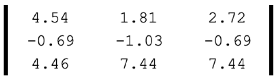
If this was a data point, it can be re-represented as a single value:

Such that this one value implies a reduction in dimensions from 9 to 1. Our illustration above reduces a matrix to its determinant, and this is loosely equivalent to dimensionality reduction.

PCA though, with eigen values & vectors, take on a slightly deeper approach. Typically, data sets that are handled under PCA are in a matrix format and the principal components, that are sought from a matrix would be a single vector column (or row) that is most significant among the other matrix vectors and would suffice as a representative of the entire matrix. As alluded in the intro above, this vector alone would hold the main components of the entire matrix, hence the name PCA. Identifying this vector though does not necessarily have to be done by eigen vectors & values, as Singular Value Decomposition (SVD) and the Power Iteration are other alternatives.

SVD is able to achieve dimensionality reduction by splitting a matrix data set into 3 separate matrices, where one of these 3, the Σ matrix, identifies the most important directions of variance in the data. This matrix that is also known as the diagonal matrix contains the singular values, which represent the magnitudes of variance along each pre-identified direction (logged in another of the 3 matrices, often referred to as U). The larger the singular value, the more significant the corresponding direction in explaining the data's variability. This leads to the U column with the highest singular value being selected as representative of the entire matrix, which does amount to reduced dimensions. From a matrix to a single vector.

Conversely, the power method iteratively refines a vector estimate to converge towards the dominant eigenvector. This eigenvector captures the direction with the most significant variation in the data and amounts to a reduced dimension of the original matrix.

However, with eigen vectors & values our focus for this article, we are able to reduce an n x n matrix into n possible n sized vectors, with each of these vectors getting assigned an Eigenvalue. This eigenvalue then informs the selection of the one eigenvector to best represent the matrix, with again a higher value indicating higher positive correlation in explaining the data variability.

So, what’s the point of reducing dimensions of data sets? In a nutshell, I feel the answer is managing white noise. However, a chattier response would be: to improve visualization, since high dimension data is more cumbersome to plot and present in media like scatter diagrams and your typical graphical formats. Reducing dimensions (plot coordinates) to 2 or 3 can help with this. Reducing computation cost in comparing data points when forecasting is another major advantage.

This comparison is done when training models, so this saves on time to train models and computing power. This leads the ‘curse of dimensionality’ where high dimensioned data tends to have accurate results when tested in sample during training, but this performance wears off more rapidly than with lower dimensioned data on cross validation. Reducing dimensions can help manage this. Also, by reducing dimensions noise in data sets tends to be reduced which in theory should improve performance. And finally, lower dimensioned data takes up less storage space and is therefore more efficient to manage especially when training large models.

PCA and Eigenvectors

Formally, eigen vectors are defined by the equation:

Av =λv

where:

• A is the transformation matrix
• v is the vector to be transformed
• a and λ is the scale factor that is applied to the vector.

Central tenet behind eigen vectors is that for many (but not all) square matrices A of a size n x n, there exists n vectors each with a size n such that the matrix A when applied to any of these vectors, the direction of the resulting product maintains the same direction as the original vector with the only change being a proportionate scale of the values in the original vector. This scale is referenced as lambda in the equation above and is better referred to as the eigen value. There is one eigen value for each eigen vector.

Not all matrices produce the required number of eigen vectors as some are deformed, however for every produced vector there is a candidate reduced dimension of the original matrix. Selection among these vectors for the winning vector is based on the eigen value, with higher values representing a better capture of the data set’s variance and less capture of its noise.

The process of identifying the eigen vector starts with normalizing the data set matrix, and quite a few options are available for this. We use z-normalization for this article. After normalizing the matrix data, the covariance matrix equivalent is then computed. Each element in the matrix captures the covariance between any two elements, with the diagonal capturing the covariance of each element with itself. Besides being more computationally efficient in calculating the eigen vectors and values when using the covariance matrix, the data values generated from the covariance matrix capture the linear relationships between the data points in the matrix and provide a clear picture of how each data point within the matrix co-varies with other data points.

Computation of the covariance matrix for matrix data types is handled by inbuilt functions in MQL5, the ‘Cov()’ function in this case. Once we have the covariance matrix, the eigen vectors and values can also be computed via the inbuilt function ‘Eig()’. Once we have the eigen vectors and their respective values, we transpose the eigen vectors matrix and multiply it with the original returns’ matrix. The rows in the matrix represent variance weighting of each portfolio and so the selected portfolio would depend on these weights. This is because its direction represents the maximum variance in data within the sampled data set.

A simple illustration to drive home the point of capturing maximum variance could be made if we take the x and y coordinates along the curve of an ellipse as a data set, with each data point having 2 dimensions x and y. If we were to plot this ellipse on a graph, it would appear as indicated below:

source 

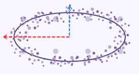
So, when tasked with the problem of reducing these x and y dimensions to a single (lower number) of dimensions, as can be seen from the plot image above clearly the x coordinate values would be a better representative of the two since the ellipse tends to stretch out a lot along its x-axis than its y-axis.

In general, though, there is a trade-off and balance to be struck between reducing dimensions and retaining information. While dimensionality reduction does have its benefits, which are listed above its interpretation and ease to explain, should be kept in mind.

Coding in MQL5

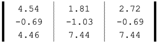
A trade system that utilizes PCA with eigen vectors typically does so by optimally selecting a portfolio from a set(s) of different iterations. To illustrate this, we can take the matrix we looked at in the introduction above to simply be a constituent of vectors, where each vector represents returns on a dollar invested for each asset under 3 different allocation regimes. The actual allocation weighting of each vector (portfolio) is only becomes important once an eigen vector is selected and the asset allocation to be adopted, in line with that vector, is then required for making future investments.

If our assets are SPY, TLT, and PDBC then its implied allocations, based on the 5 year returns for each of these ETFs is:

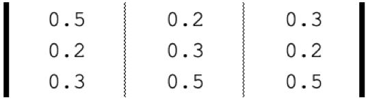
So what PCA with eigen vectors would do is help us select an ideal portfolio (asset allocation) among these 3 options based on their performance over the past 5 years. If we recount the steps outlined above, the first thing we need to do is always normalize the data set and as mentioned we are using z-normalization for this and the source code to do it is below:

//+------------------------------------------------------------------+
//| Z-Normalization                                                  |
//+------------------------------------------------------------------+
matrix ZNorm(matrix &M)
{  matrix _z;
   _z.Init(M.Rows(), M.Cols());
   _z.Copy(M);
   if(M.Rows() > 0 && M.Cols() > 0)
   {  double _std_min = (M.Max() - M.Min()) / (M.Rows() * M.Cols());
      if(_std_min > 0.0)
      {  double _mean = M.Mean();
         double _std = fmax(_std_min, M.Std());
         for(ulong i = 0; i < M.Rows(); i++)
         {  for(ulong ii = 0; ii < M.Cols(); ii++)
            {  _z[i][ii] = (M[i][ii] - _mean) / _std;
            }
         }
      }
   }
   return(_z);
}

Once we normalize the returns matrix, we would then compute the covariance matrix of what we’ve normalized. MQL5’s in built data type for matrix can handle this for us in one line:

   matrix _z = ZNorm(_m);
   matrix _cov_col = _z.Cov(false);

Armed with the covariance relations of each data point within the matrix we can then work out the eigen vectors and eigen values. This also is a single line:

   matrix _e_vectors;
   vector _e_values;
   _cov_col.Eig(_e_vectors, _e_values);

The output from the above function is two-fold and our interest is primarily in the eigen vectors which are returned as a matrix. This matrix when transposed and multiplied with the original returns’ matrix presents us with what we are looking for, the projection matrix P. This is a matrix with rows for each of the possible portfolios where the column in each row represents a weighting to each of the 3 generated eigen vectors. For instance, in the first row the largest value is in the first column. This means most of this portfolio’s variance in returns is attributable to the first eigen vector. If we look at the eigen value of this eigen vector we can see it is the largest of the three. This therefore implies that across all three portfolios the first one accounts for the majority of the significant patterns (or trends) represented in the data matrix.

In our case all portfolios were yielding positive returns if their values are summed up by column, since each column represents a portfolio. In fact, the only negative returns are from holding the bonds ETF PDBC regardless of one’s allocation. This means that if one wants to ‘perpetuate’ these hedged or diversified or good-beta returns he would need to stick to portfolio 1. Once again, the overall theme from the returns data matrix is for positive returns in equities and commodities and negative returns from bonds. So, PCA with eigen vectors can filter out a portfolio from these that is most likely to continue this trend, as is the case with portfolio 1 or one to even do the reverse which in our case would be portfolio 3 since in the projection matrix the 3^rd row’s maximum value is in column 3 and the 3^rd eigen vector had the least value.

Noteworthy is that this portfolio does not have the best returns and this process does not select this per se. All that it does is provide indicative weighting on maintaining the status quo. It all sounds unnecessarily complex for a selection that could easily be made on inspection and yet as returns or analyzed matrices get larger with more rows and columns (PCA with eigen vectors requires square matrices) then this process does start to pay off.

To showcase PCA in a signal class we are constrained in that by default only one symbol on a single timeframe can be tested which means the notions we had above on portfolio selection are not applicable out of the box. There are work-arounds these constraints and perhaps we could cover them in another article in the future but for now we will work within these limitations.

What we’ll do is analyze for a single symbol on the daily timeframe, price changes for every day of the week. Since there are 5 trade days in a week, our matrix will have 5 columns and in order to get the 5 rows required for PCA eigen vector analysis we will consider 5 different price types namely: Open, High, Low, Close, and Typical. Determining the eigen vectors and values will follow the steps already mentioned above.

The same applies to getting the projection matrix, and once we have it we can easily read-off the trade day of the week and applied price type that capture the most variance. If we follow the script listing below:

   matrix _t = _e_vectors.Transpose();
   matrix _p = _m * _t;
   //Print(" projection: \n", _p);
   vector _max_row = _p.Max(0);
   vector _max_col = _p.Max(1);
   double _days[];
   _max_row.Swap(_days);
   PrintFormat(" best trade day is: %s", EnumToString(ENUM_DAY_OF_WEEK(ArrayMaximum(_days)+1)));
   ENUM_APPLIED_PRICE _price[__SIZE];
   _price[0] = PRICE_OPEN;
   _price[1] = PRICE_WEIGHTED;
   _price[2] = PRICE_MEDIAN;
   _price[3] = PRICE_CLOSE;
   _price[4] = PRICE_TYPICAL;
   double _prices[];
   _max_col.Swap(_prices);
   PrintFormat(" best applied price is: %s", EnumToString(_price[ArrayMaximum(_prices)]));
   PrintFormat(" worst trade day is: %s", EnumToString(ENUM_DAY_OF_WEEK(ArrayMinimum(_days)+1)));
   PrintFormat(" worst applied price is: %s", EnumToString(_price[ArrayMinimum(_prices)]));

Our print log outputs are indicated below under strategy testing and results.

So, from our logs above we can see that Thursdays and Closing-price series are responsible for most of the variance in the price action of the symbol on whose chart the script is attached (the script was attached to EURJPY). So, what does this mean? It implies if one finds the overall trend and price action of EURJPY interesting and he would like to make similar plays going forward then he would be better off focusing his trades on Thursday and use Close-price series. Supposing EURJPY was part of a set position in one’s portfolio and going forward exposure to EURJPY was being scaled down how would the position matrix help? The ‘worst’ trade days and price series could be used in determining when and how to close positions of EURJPY.

So, our position matrix recommends trade days and price series so let’s use the simple signal class below that takes these into account.

   int _buffer_size = CopyRates(Symbol(), Period(), __start, __stop, _rates);
   PrintFormat(__FUNCSIG__+" buffered: %i",_buffer_size);
   if(_buffer_size >= 1)
   {  for(int i = 1; i < _buffer_size - 1; i++)
      {  TimeToStruct(_rates[i].time,_datetime);
         int _iii = int(_datetime.day_of_week)-1;
         if(_datetime.day_of_week == SUNDAY || _datetime.day_of_week == SATURDAY)
         {  _iii = 0;
         }
         for(int ii = 0; ii < __SIZE; ii++)
         {  
                ...

                ...
         }
      }
   }

Strategy Testing and Results

To perform our back tests with an expert advisor assembled in the MQL5 wizard, we first need to run the script on the chart and time frame of the symbol that we’ll be testing. For our illustration, that is EURUSD on the 4-hour time frame. If we run the script on the chart, we get Friday and the Weighted Price as the ‘ideal’ or variance determining parameters for EURUSD on the 4-hour. This is indicated in the logs below:

2024.04.15 14:55:51.297 ev_5 (EURUSD.ln,H4)      best trade day is: FRIDAY
2024.04.15 14:55:51.297 ev_5 (EURUSD.ln,H4)      best applied price is: PRICE_WEIGHTED
2024.04.15 14:55:51.297 ev_5 (EURUSD.ln,H4)      worst trade day is: TUESDAY
2024.04.15 14:55:51.297 ev_5 (EURUSD.ln,H4)      worst applied price is: PRICE_OPEN

Our script also has 2 input parameters that determine the period under analysis, namely the start time and stop time. Both are datetime variables. We set these to 2022.01.01 and 2023.01.01 so that we can first test our expert advisor on this period and then cross validate in with the same settings on the period from 2023.01.01 to 2024.01.01. The script recommends Friday and Weighted Price as the best variance determining variables, so, how do we use this information in developing a signal class? There are a number of options, as always, that one can consider what we will look at though is the simple price – moving average cross over indicator. By using the moving average of the recommended applied price, and also by placing trades only on the recommended weekday we’ll attempt to cross validate the thesis presented from our script. The code therefore for our expert signal class will be very simple, and this is shared below:

//+------------------------------------------------------------------+
//| "Voting" that price will grow.                                   |
//+------------------------------------------------------------------+
int CSignalPCA::LongCondition(void)
{  int _result = 0;
   m_MA.Refresh(-1);
   m_close.Refresh(-1);
   m_time.Refresh(-1);
//
   if(m_MA.Main(StartIndex()+1) > m_close.GetData(StartIndex()+1) && m_MA.Main(StartIndex()) < m_close.GetData(StartIndex()))
   {  _result = 100;
      //PrintFormat(__FUNCSIG__);
   }
   if(m_pca)
   {  TimeToStruct(m_time.GetData(StartIndex()),__D);
      if(__D.day_of_week != m_day)
      {  _result = 0;
      }
   }
//
   return(_result);
}
//+------------------------------------------------------------------+
//| "Voting" that price will fall.                                   |
//+------------------------------------------------------------------+
int CSignalPCA::ShortCondition(void)
{  int _result = 0;
   m_MA.Refresh(-1);
   m_close.Refresh(-1);
//
   if(m_MA.Main(StartIndex()+1) < m_close.GetData(StartIndex()+1) && m_MA.Main(StartIndex()) > m_close.GetData(StartIndex()))
   {  _result = 100;
      //PrintFormat(__FUNCSIG__);
   }
   if(m_pca)
   {  TimeToStruct(m_time.GetData(StartIndex()),__D);
      if(__D.day_of_week != m_day)
      {  _result = 0;
      }
   }
//
   return(_result);
}

As always, we do not use price targets for take profit or stop loss and strictly use limit order entry. This implies once a position is opened by our expert advisor, it only gets closed on reversal; an arguably high-risk approach, but for our purposes it will suffice. If we perform back tests on the first period, we do get the following report and equity curve:

The above results are from 2022.01.01 to 2023.01.01. If we attempt to test with the same settings over a longer period that extends beyond the script analysis period by running from 2022.01.01 to 2024.01.01, we get the following results:

Our expert signal is a bit restrictive and not too many trades are placed, which one could argue does not amount to sufficient testing. Regardless though test periods of a few years are not reliable when considering live account runs. As a control, besides the cross validation above, we can also run tests on different applied prices while trading on any day of the week with the same expert advisor settings. This does produce the following results:

The overall performance clearly suffers once we stray beyond the PCA script recommendation, but why is this? Why does trading only within the variance determining parameters give us better results than the unconstrained setups? This I feel is a relevant question because influencing the variance does not necessarily imply more profitability since the overall trend of the data set under study could be whipsawed. This is why selecting the most variance determining settings should only be done if the underlying and overall trends in the data set under study are consistent with the overall objectives of the trader.

If we examine the EURUSD price chart we can see in the PCA analysis period of 2022.01.01 to 2023.01.01, EURUSD was mostly trending lower before in briefly reversed in October. However, in the cross-validation period, 2023, the pair whipsawed a lot without making any major trends like in 2022. This could imply that by performing analyses over major trend periods, the trend setting variance parameters can better be captured, and they could be useful even in whipsaw situations, as is evident in 2023.

Conclusion

To sum up we have seen how PCA is inherently an analysis tool that seeks to reduce data set(s) dimensionality by identifying the dimensions (or components of the data set) that are most responsible for determining its underlying trends. There are many available tools for reducing data dimensionality and on the surface PCA may seem jejune but it does require cautious analysis and interpretation given that it is always based on the underlying trends of the studied data set.

In the example we looked under testing the underlying trends for the studied symbol were bearish and based on this in cross-validation majority of the out of sample trades placed were short. If hypothetically we had studied a bullish market for the symbol under consideration then any trade strategies to be adopted based on the recommended PCA settings would have to capitalize on a bullish environment. Conversely in those situations it could make sense to choose settings that least explain the variance if one intends to capitalize on a bearish market since a bearish market and a bullish market are polar opposites. And also, PCA yields more than one pair of settings each with a weighting aka eigen value implying more than one setting can be adopted if their weightings are above a sufficient threshold. This has not been explored in this article and the reader is welcome to look into this as the source code is attached below. The use of this code in the MQL5 wizard to assemble an expert advisor can be looked up here for those new to the wizard.

However, one of the approaches one can take in accommodating more PCA settings within the analysis script and expert adviser would simply be by firstly normalizing the eigen values such that, for example, they are all positive and in the range 0.0 to 1.0. Once this is done you can then define selection thresholds for the eigen vectors you will pick from each analysis. For example, if a PCA analysis of a 3 x 3 matrix initially gives the values 2.94, 1.92, 0.14 then we would normalize these values to a 0 – 1 range as: 0.588, 0.384, & 0.028. With the normalized values a threshold benchmark like 0.3 can allow one to impartially select eigen vectors across multiple analyses. A repeat analysis with a different data set and even different matrix size can still have its eigen vectors selected in a similar fashion. For the script this would mean iterating through the eigen values and adding the 2 cross properties for each matched value, to an output list or array. This array could be a struct that logs both the ‘x’ and ‘y’ properties in the data set matrix. With the expert adviser you would need to have the filter properties inputted as string values separated by a comma, for scalability. This would require parsing the string and extracting the properties, into a standard format readable by the Expert Advisor.