MQL5 Wizard Techniques You Should Know (Part 15): Support Vector Machines with Newton's Polynomial

Introduction

Support Vector Machines (SVM) is a machine learning classification algorithm. Classification is different from clustering which we have considered in previous articles here and here with the primary difference between the two being that classification separates data into predefined sets, with supervision, while clustering seeks to determine what and how many of these sets there are, without supervision.

In a nutshell, SVM classifies data by considering the relationship each data point will have with all the others, if a dimension were to be added to the data. Classification is achieved if a hyperplane, can be defined that cleanly dissects the predefined data sets.

Often the data sets under consideration have multiple dimensions, and it is this very attribute that makes SVM a very powerful tool in classifying such data sets, especially if the numbers in each set is small or the relative proportion of the data sets is skewed. The implementation source code for SVMs that have more than 2 dimensions is very complex and often use cases in python or C# always uses libraries, leaving the user with minimum code input to get a result.

High dimensioned data has a tendency to curve-fit training data, a lot which makes it less reliable in out of sample data and this is one main drawbacks to SVM. Lower dimensioned data, on the other hand, does cross-validate much better, and have more common use cases.

For this article we will consider a very basic SVM case that handles 2-dimensional data (also known as linear-SVM), since complete implementation source code is to be shared without reference to any 3^rd party libraries. Usually, the separating hyperplane is derived from either one of two methods: a polynomial kernel or a radial kernel. The latter is more complex and will not be discussed here as we will be dealing only with the former, the polynomial kernel.

Typically, when using the polynomial kernel, that is formally defined by the equation below,

determining the ideal c and d values, which set the equation of the hyperplane, is an iterative process that aims to have support vectors as far apart as possible since they measure the gap between the two data sets.

For this article though, as indicated in the title, we will use Newton’s Polynomial in deriving the equation of the hyperplane on 2-dimensional data sets. We had looked at Newton’s Polynomial in a recent article, so some of its implementation will be skimmed over.

We implement Newton’s Polynomial (NP) in three scenarios. First, we interpolate mid-points between two predefined data sets to get a boundary set of points and these points are used to derive a line/ curve equation that defines our hyperplane. With this hyperplane defined, we treat it as a classifier in executing trade decisions for a test expert signal class, to be used. In the second scenario we add a regression function so that the expert signal class no outputs of only 0 or 100 values (as in the 1^st) but provides values between the range as well. We compute the regression value from how close the unclassified vector is from the known vector points. Thirdly, we build on the second scenario by interpolating only a small number of points when defining the hyperplane. The small number of points, aka support vectors, being those closer to the other data set, thus ‘refining’ the hyperplane equation while adopting everything else.

Background on the Polynomial Kernel

For this piece we are considering linear SVMs given that the complete source code implementation is to be shared, and we want to avoid using libraries by offering complete transparency on all source code. In real-world applications of SVM, though, the non-linear types get used a lot, given the inherent complexity and multidimensionality of many data sets. Dealing with these challenges in SVMs has proven manageable thanks to the kernel trick. This is a method that allows a data set to be studied at a higher dimension while maintaining its original structure. The kernel trick uses dot product of vectors to preserve the lower dimension vector values. In pointing the data set to higher dimensions, separation of the data sets is easily achieved and this is done with less compute resources as well.

As indicated above, our kernel function is formally defined as:

with x and y serving as data points across any two compared data points in each set, c being a constant (whose value is often set to 1 initially) and d being the polynomial degree. As d increases a more accurate hyperplane equation can be defined, but this tends to lead to over fitting, a balance needs to be set. The x and y data points are in many cases in vector or even matrix format, which is why the power T represents the transpose of x.

Implementing a polynomial kernel in MQL5, for illustration purposes, could take the following form.

//+------------------------------------------------------------------+
//| Define a data point structure                                    |
//+------------------------------------------------------------------+
struct Sdatapoint
{  double      features[2];
   int               label;
                     Sdatapoint()
   {                 ArrayInitialize(features, 0.0);
      label = 0;
   };
                    ~Sdatapoint() {};

};

//+------------------------------------------------------------------+
//| Function to calculate the polynomial kernel value                |
//+------------------------------------------------------------------+
double PolynomialKernel(Sdatapoint &A, Sdatapoint &B, double Constant, int Degree)
{  double _kernel_sum = 0.0;
   for (int i = 0; i < 2; i++)
   {  _kernel_sum += (A.features[i] * B.features[i]);
   }
   _kernel_sum += Constant; // Add constant term
   return(pow(_kernel_sum, Degree));
}

Relationship weights between data points that are in separate sets are computed and stored in a kernel matrix. This kernel matrix quantifies data point spacing and therefore filters out for the support vectors, the data points at the edge of each data set and are closer to the neighboring set.

source

These support vectors then serve as an input computing the hyperplane equation. All this is handles in library functions like: PyLIBSVM, or shogun for python; or kernlab or SVMlight in R. It is library functions such as these, given the complex nature of deriving the hyperplane equation, that do compute and output the hyperplane.

When determining the kernel matrix, various constant and polynomial degree values can be considered in arriving at an optimal solution. Because this though makes an already complex process of deriving a hyperplane from just one matrix even more complicated by doing this over multiple matrices, it is more prudent to always select a definitive (or suboptimal from know-how) constant and polynomial degree once at the beginning and use that to arrive at the hyperplane. To this end, the constant value is also often set as 1. And as one might expect, the higher the degree polynomial the better the classification, but this has risks of over fitting already mentioned to above.

Also, higher polynomial degrees tend to be more computationally intense, so an intuitive value that is not too high needs to be established at the onset.

Polynomial kernels which are considered here are relatively easy to understand, but they are not the most used or preferred kernel in many SVM implementations as those bragging rights go to the radial basis function kernel.

The radial basis function (RBF) kernel is more commonly chosen because SVM’s edge is in handling multi-dimensional data and RBF kernel excels at this better than the polynomial kernel. Once a kernel is chosen, the dual optimization problem, where, as mentioned above the data sets get mapped to a higher dimension space, would be undertaken and thanks to dot product rules that are captured in what is referred to as the kernel trick this optimization (back and forth) can be done more efficiently while also being expressed more plainly. The complex nature of hyperplane equations for data sets with more than 2 dimensions make this indispensable. When all is said and done the hyperplane equation does take the following form:

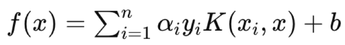
where:

• f(x) is the decision function.
• αi​ are the coefficients obtained from the optimization process.
• yi​ are the class labels.
• K(xi​,x) is the kernel function.
• b is the bias term.

The hyperplane equation defines how the two data sets are separated by the decision function assigning a class label which defines which side any query point belongs to. So, a query data point would be the x in the equation with xi and yi being the train data and its classifiers respectively.

As an aside, applications of SVM are vast, and they can range from: spam filtering if you can embed email headers and content into a structured format; screening loan applicants against default; etc. What would make SVM ideal as opposed to other machine learning alternatives is the robustness to develop models from small or very skewed data sets.

Implementing in MQL5

The model struct we use for storing x and y values is very similar to our recent implementations with the difference here being the addition of a counter for each classifier type. SVM is inherently a classifier, and we will look at examples of this in action where these counters will be handy.

So, the x vector values are 2 at each index, since we are restricting the multi-dimensionality of our data sets to 2 so as to be able to use the Newton’s Polynomial. Increased dimensionality also risks over fitting. The first dimension or value of x is the changes in high price buffer, while the second will be changes in low price buffer as one would expect. The choice of input data is now a crucial aspect in machine learning. Although transformers, CNNs, and RNNs are very resourceful, the decision on input data and how you embed or normalize them can be more critical.

. We have chosen a very simple data set, but the reader should be aware that his choice of input data is not limited to raw price data or even indicator values, but it could include news economic indicator values. And again, how you choose to normalize this can make all the difference.

//+------------------------------------------------------------------+
//| Function to get and prepare data.                                |
//+------------------------------------------------------------------+
double CSignalSVM::GetOutput(int Index)
{  double _get = 0.0;
   

        ....
        ....

   int _x = StartIndex() + Index;
   for(int i = 0; i < m_length; i++)
   {  for(int ii = 0; ii < Dimensions(); ii++)
      {  if(ii == 0) //dim-1
         {  m_model.x[i][ii] = m_high.GetData(StartIndex() + i + _x) - m_high.GetData(StartIndex() + i + _x + 1);
         }
         else if(ii == 1) //dim-2
         {  m_model.x[i][ii] = m_low.GetData(StartIndex() + i + _x) - m_low.GetData(StartIndex() + i + _x + 1);
         }
      }
      if(i > 0) //assign classifier
      {  if(m_close.GetData(StartIndex() + i + _x - 1) - m_close.GetData(StartIndex() + i + _x) > 0.0)
         {  m_model.y[i - 1] = 1;
            m_model.y1s++;
         }
         else if(m_close.GetData(StartIndex() + i + _x - 1) - m_close.GetData(StartIndex() + i + _x) < 0.0)
         {  m_model.y[i - 1] = 0;
            m_model.y0s++;
         }
      }
   }
//
   _get = SetOutput();
   return(_get);
}

Our y data set, will be forward lagged changes in the close price, as has been the case previously. We introduce counters for the two classes that are labelled ‘y0’ and ‘y1’. These simply log, for each processed bar whose two x values are established, whether the subsequent change in the close price was bullish (in which case a 0 is logged) or it was bearish (where a 1 would be recorded).

Since y is a vector, we could have as a side note retrieved these 0 and 1 counts by comparing its current values to vectors filled with 0s and vectors filled with 1s as the returned values would effectively be a count present 0s and 1s in the y vector respectively.

The ‘set-output’ function is another addition to the functions we’ve had, in processing our model information. It takes x vector values for each class, and interpolates a mid-point between the two sets that could serve as a hyperplane of the two sets. This is not the SVM approach as already mentioned but what this does for us, since we want to define a hyper plane by Newton’s Polynomial, is give us a set of points that we can work with to derive a hyperplane equation.

//+------------------------------------------------------------------+
//| Function to set and train data                                   |
//+------------------------------------------------------------------+
double CSignalSVM::SetOutput(void)
{  double _set = 0.0;
   matrix _a,_b;
   Classifier(_a,_b);
   if(_a.Rows() * _b.Rows() > 0)
   {  matrix _interpolate;
      _interpolate.Init(_a.Rows() * _b.Rows(), Dimensions());
      for(int i = 0; i < int(_a.Rows()); i++)
      {  for(int ii = 0; ii < int(_b.Rows()); ii++)
         {  _interpolate[(i*_b.Rows())+ii][0] = 0.5 * (_a[i][0] + _b[ii][0]);
            _interpolate[(i*_b.Rows())+ii][1] = 0.5 * (_a[i][1] + _b[ii][1]);
         }
      }
      vector _w;
      vector _x = _interpolate.Col(0);
      vector _y = _interpolate.Col(1);
      _w.Init(m_model.y0s * m_model.y1s);
      _w[0] = _y[0];
      m_newton.Set(_w, _x, _y);
      double _xx = m_model.x[0][0], _yy = m_model.x[0][1], _zz = 0.0;
      m_newton.Get(_w, _xx, _zz);
      if(_yy < _zz)
      {  _set = 100.0;
      }
      else if(_yy > _zz)
      {  _set = -100.0;
      }
      _set *= Regressor(_x, _y, _xx, _yy);
   }
   return(_set);
}

We are considering 3 approaches at deriving the hyperplane within this method. The very first approach considers all points in each set in coming up with the hyperplane points by interpolating the mean of each point in a set to every point in the alternative set. This clearly is not considering support vectors but is presented here for study and comparison purposes with the other approaches.

The second method is similar to the first with the only difference being that the forecast y value is regressed, meaning rather than have it as a 0 or 1 we use a ‘regulizer’ function to transform or normalize the output forecasts as a floating-point value in the range 0.0 to 1.0. This effectively produces a system which in principle is further still from SVMs, but still uses a hyperplane to differentiate 2-dimensional data points.

//+------------------------------------------------------------------+
//| Regressor for the model                                          |
//+------------------------------------------------------------------+
double CSignalSVM::Regressor(vector &X, vector &Y, double XX, double YY)
{  double _x_max = fmax(X.Max(), XX);
   double _x_min = fmin(X.Min(), XX);
   double _y_max = fmax(Y.Max(), YY);
   double _y_min = fmin(Y.Min(), YY);
   return(0.5 * ((1.0 - ((_x_max - XX) / fmax(m_symbol.Point(), _x_max - _x_min))) + (1.0 - ((_y_max - YY) / fmax(m_symbol.Point(), _y_max - _y_min)))));
}

We are able to get a proxy regressive value by comparing the forecast value to the maximum and minimum, value in its set such that if it matches the minimum 0 is returned versus 1 that would be returned if it was matching the maximum value.

Thirdly and finally, we improve the method in part 2 by adding a ‘classifier’ function that filters the points in each of the sets that are used in deriving the hyperplane. By considering points that are furthest from the centroid of their own set while being closest to the centroid of the opposing set, we come up with 2 subsets of points, one from each class, that can be used to interpolate the hyperplane boundary between the two sets.

//+------------------------------------------------------------------+
//| 'Classifier' for the model that identifies Support Vector points |
//|  for each set.                                                   |
//+------------------------------------------------------------------+
void CSignalSVM::Classifier(matrix &A, matrix &B)
{  if(m_model.y0s * m_model.y1s > 0)
   {  matrix _a_centroid, _b_centroid;
      _a_centroid.Init(1, Dimensions());
      _b_centroid.Init(1, Dimensions());
      for(int i = 0; i < m_length; i++)
      {  if(m_model.y[i] == 0)
         {  _a_centroid[0][0] += m_model.x[i][0];
            _a_centroid[0][1] += m_model.x[i][1];
         }
         else if(m_model.y[i] == 1)
         {  _b_centroid[0][0] += m_model.x[i][0];
            _b_centroid[0][1] += m_model.x[i][1];
         }
      }
      _a_centroid[0][0] /= m_model.y0s;
      _a_centroid[0][1] /= m_model.y0s;
      _b_centroid[0][0] /= m_model.y1s;
      _b_centroid[0][1] /= m_model.y1s;
      double _a_sd = 0.0, _b_sd = 0.0;
      double _ab_sd = 0.0, _ba_sd = 0.0;
      for(int i = 0; i < m_length; i++)
      {  if(m_model.y[i] == 0)
         {  double _0 = 0.0;
            _0 += pow(_a_centroid[0][0] - m_model.x[i][0], 2.0);
            _0 += pow(_a_centroid[0][1] - m_model.x[i][1], 2.0);
            _a_sd += sqrt(_0);
            double _1 = 0.0;
            _1 += pow(_b_centroid[0][0] - m_model.x[i][0], 2.0);
            _1 += pow(_b_centroid[0][1] - m_model.x[i][1], 2.0);
            _ab_sd += sqrt(_1);
         }
         else if(m_model.y[i] == 1)
         {  double _1 = 0.0;
            _1 += pow(_b_centroid[0][0] - m_model.x[i][0], 2.0);
            _1 += pow(_b_centroid[0][1] - m_model.x[i][1], 2.0);
            _b_sd += sqrt(_1);
            double _0 = 0.0;
            _0 += pow(_a_centroid[0][0] - m_model.x[i][0], 2.0);
            _0 += pow(_a_centroid[0][1] - m_model.x[i][1], 2.0);
            _ba_sd += sqrt(_0);
         }
      }
      _a_sd /= m_model.y0s;
      _ab_sd /= m_model.y0s;
      _b_sd /= m_model.y1s;
      _ba_sd /= m_model.y1s;
      for(int i = 0; i < m_length; i++)
      {  if(m_model.y[i] == 0)
         {  double _0 = 0.0;
            _0 += pow(_a_centroid[0][0] - m_model.x[i][0], 2.0);
            _0 += pow(_a_centroid[0][1] - m_model.x[i][1], 2.0);
            double _1 = 0.0;
            _1 += pow(_b_centroid[0][0] - m_model.x[i][0], 2.0);
            _1 += pow(_b_centroid[0][1] - m_model.x[i][1], 2.0);
            if(sqrt(_0) >= _a_sd && _ab_sd <= sqrt(_1))
            {  A.Resize(A.Rows()+1,Dimensions());
               A[A.Rows()-1][0] = m_model.x[i][0];
               A[A.Rows()-1][1] = m_model.x[i][1];
            }
         }
         else if(m_model.y[i] == 1)
         {  double _1 = 0.0;
            _1 += pow(_b_centroid[0][0] - m_model.x[i][0], 2.0);
            _1 += pow(_b_centroid[0][1] - m_model.x[i][1], 2.0);
            double _0 = 0.0;
            _0 += pow(_a_centroid[0][0] - m_model.x[i][0], 2.0);
            _0 += pow(_a_centroid[0][1] - m_model.x[i][1], 2.0);
            if(sqrt(_1) >= _b_sd && _ba_sd <= sqrt(_0))
            {  B.Resize(B.Rows()+1,Dimensions());
               B[B.Rows()-1][0] = m_model.x[i][0];
               B[B.Rows()-1][1] = m_model.x[i][1];
            }
         }
      }
   }
}

The code shared above that does this is a bit lengthy and am sure more efficient implementations of this can be done, especially if one were to engage the inbuilt functions of the vector and matrix data types that were recently introduced in MQL5. But what we are doing is first finding the centroid (or average) of each data set. Once that is defined, we proceed to work out each data set’s standard deviation and this is got by the variables that are suffixed ‘_sd’. Once armed with centroid coordinates and standard deviation magnitude we can measure and compare for each point how far it is from its centroid as well as how far it is from the centroid of the opposing data set with the computed standard deviations serving as a threshold for being too far or too close.

Interpolated points are all we need to define an equation with the Newton’s polynomial. As we saw here, the more points one provides, the higher the equation exponent. The maximum number of interpolated points we can use with Newton’s Polynomial is controlled by the size of the data sets and this is directly proportional to the ‘m_length’ parameter, a variable that sets how many data points in history we need to look back when defining the two data sets in the model.

Of the three methods used to derive a hyperplane, only the last bears any semblance to the typical SVM methods. By screening for points within each set, that are closest to the set's boundary and are therefore more relevant to the hyperplane, we are defining the support vectors. These support vector points then serve as input to our Newton Polynomial class in deriving the hyperplane equation. By contrast, if we were to do a strict SVM, we would add an extra dimension to our data points for extra differentiation while iterating through the constants in the polynomial kernel equation which enables this. Even with only 2-dimensional data it is clearly an order of magnitude more complicated not to mention the compute resources involved. In fact, for simplicity or best practice, one of these constants (the c) is always assumed to be 1, while only the polynomial degree variable (the d in the equations above) gets optimized. And as you can imagine with data sets that have more than 2 dimensions this would clearly necessitate a 3^rd party library because if nothing else the 4, 5, or nth exponent equation that is sought will be some orders of magnitude more complex.

The Newton Polynomial implementation is very similar to what we covered in the previous related article, save for some debugging on the ‘Get’ function which runs the built equation to determine the next y value. This is attached below.

Tester Results

The 3 signal class files attached at the end of this article can each be assembled into an expert advisor via the MQL5 wizard. Examples on how this is done are available in articles here and here.

So, on running tests for the very first implementation where the hyperplane is got from interpolating across all points in either set without screening for support vectors does give us the following results:

If we do similar test runs, as above where our test symbol is EURJPY on the daily time frame for the year 2023, for the second method which only adds regression to the method above we have the following:

Finally, the approach with the most semblance to SVM which screens either data set for support vector points before deriving its hyperplane, when tested gives us the following results:

From our reports above it may, from a quick scan, be surmised that the method that uses support vectors is the most promising and that should probably not be a surprise given the extra fine-tuning (even though the number of parameters is identical in all three methods) involved.

As a side note, this testing is performed on real ticks with limit orders and no profit targets or stop losses are used. As always, more testing is necessary prior to drawing more meaningful conclusions. However, it is interesting to note that, with the same number of input parameters, the support vector method performs better. It made fewer trades and that gave drastically better performance than the other two approaches.

Adding regression in the second approach only marginally improved performance, as can be seen from the results. The number of trades was also almost the same, however pre-screening the data set points for support vectors prior to defining the hyperplane was clearly a game changer. MetaTrader reports are very subjective with many debating what would be the most critical statistic to rely on as an indicator on whether the trade system can walk forward, and I do not have a definitive answer on that topic as well. However, I think that a comparison between the average profit and average loss (per trade) while also minding average consecutive wins to average consecutive loss ratio could be insightful. All these values are often combined in calculating a ratio referred to as the expectancy. This is very different from the expected payoff, which is simply the profit divided by all trades. If we compare the expectancy of all reports, then the method that used support vectors is better by a magnitude of almost 10 when compared to the other 2 approaches.

Conclusion

So, to sum up, we have looked at another example of quickly developing and testing a possible trade idea to assess if it is an improvement, or a fit within one’s existing strategy.

SVM is a fairly complicated algorithm that is seldom if at all implemented without the help of a 3^rd party library whether that be PyLIBSVM for python or SVMlight for R and more than that one of the optimizable parameters is often taken to be equal to be 1 to simplify this process. To recap, this process, a copy of a data set under study gets its dimensions increased via a specific reversible formula referred to as the polynomial kernel. It is the relative simplicity and reversibility of this polynomial kernel that earns it the name the ‘kernel trick’. This simplicity and reversibility, that is possible thanks to dot products, is much needed in cases where the data set has more than 2 dimensions because as one can imagine in cases of data sets with very high dimensionality, the hyperplane equation that properly classifies such data sets is bound to be very complex.

So, by introducing an alternative way at deriving the hyperplane via Newton’s Polynomial that firstly is not as compute intense but also is much better to understand and present; variant implementations of SVM can not only be tested, but they could be considered either as alternatives to one’s existing strategy or as accretive. The MQL5 IDE allows both scenarios, were in the former you’d develop an entirely new trade system based on the signal class code shared here. But perhaps what is often overlooked is the accretive potential presented by the MQL5 wizard that allows the assembly and testing of multiple strategies concurrently. This too can be done quickly and with minimal coding when screening for ideas and strategies at the preliminary stage. And as always, besides looking at the signal class of the wizard assembled classes, the trailing class and money management classes can be explored as well.