
Neural networks made easy (Part 52): Research with optimism and distribution correction

Introduction
One of the basic elements for increasing the stability of Q-function learning is the use of an experience replay buffer. Increasing the buffer makes it possible to collect more diverse examples of interaction with the environment. This allows our model to better study and reproduce the Q-function of the environment. This technique is widely used in various reinforcement learning algorithms, including algorithms of the Actor-Critic family.
But there is also another side to the coin. During the learning process, the Actor's actions become increasingly different from the examples stored in the experience replay buffer. The more iterations of updating the model parameters, the greater this difference. This leads to a decrease in the efficiency of training the Actor policy. One possible solution was presented in the article "Off-policy Reinforcement Learning with Optimistic Exploration and Distribution Correction" (October 2021). The authors of the method proposed adapting the Distribution Correction Estimation (DICE) method to the Soft Actor-Critic algorithm.
At the same time, the method authors paid attention to yet another nuance. While training the policies, the Soft Actor-Critic method uses minimal action evaluation. The practical use of this approach demonstrates a tendency towards pessimistic insufficient research of the environment and directed homogeneity of actions. To minimize this effect, the authors of the article proposed additionally training an optimistic research Actor model. This, in turn, further increases the gap between the example of interaction between the optimistic Actor model and the environment and the distribution of actions of the trained target model.
However, the combined use of correction of distribution estimates and the study of an optimistic Actor model can improve the training result of the target model.

1. Research with optimism
The first ideas about environmental research with optimism were stated in the article "Better Exploration with Optimistic Actor-Critic" (October 2019). Its authors noticed that the combination of the actor’s greedy updating with the critic’s pessimistic assessment leads to the avoidance of actions the agent does not know about. This phenomenon has been called "pessimistic underexploration". In addition, most algorithms are not informed about the research direction. Randomly sampled actions are equally likely to be located on opposite sides of the current average, while we generally need actions in certain areas much more than others. To correct these phenomena, the Optimistic Actor Critic (OAC) algorithm was proposed, which approximates the lower and upper confidence bounds of the state-action value function. This allowed the principle of optimism to be used in the uncertainty of performing directed research using an upper bound. At the same time, the lower limit helps to avoid overestimating actions.
The method authors picked up and developed the ideas of Optimistic Actor Critic. As in Soft Actor-Critic, we will train 2 Critic models. But at the same time, we will also train 2 Actor models: πе and target πт research.
The πе policy learns to maximize the approximate upper bound of the QUB Q-function values. At the same time, πт maximizes the approximation of the lower bound of the QLB Q-function during training. OAC shows that the research involving πе allows reaching more efficient use of sampling compared to Soft Actor-Critic.
To obtain an approximate upper bound of the QUB Q-function, the mean and variance of the ratings of both Critics are calculated first:
![]()
Next, we define QUB using the equation:
![]()
where βUB ∈ R and manages the optimism level.
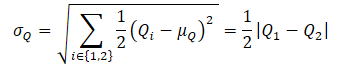
Note that the previous approximate lower bound of the QLB Q-function can be expressed as
![]()
At the pessimism level of βLB = 1 QLB equals the minimum of the Critics' ratings.
Optimistic Actor-Critic applies a maximum KL divergence constraint between πе and πт, which allows us to obtain a closed solution for πе and stabilizes training. At the same time, this limits the potential of πе in performing more informative actions that could potentially correct critics’ false assessments. This restriction does not allow πе generate actions that are very different from those generated by the πт policy trained conservatively based on the minimum evaluation of critics.
In the SAC+DICE algorithm, the addition of distribution correction eliminates the use of the KL constraint to unlock all exploration possibilities with an optimistic policy. In this case, the stability of training is maintained by explicitly correcting the biased gradient estimate when training the policy.
While training the Actor's behavioral policy πт to prevent overestimation of the Q-function, an approximate lower bound of QLB is used as a critic, as in the Soft Actor-Critic method. However, an adjustment to the sampling distribution is added using the dπт(s,a)/dD(s,a) ratio. We get the following training goal:
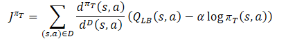
where dπт(s,a) represents the state-action distribution of the current policy, while dD(s,a) defines the state-action distribution from the experience playback buffer. The gradient of such a training target provides an unbiased estimate of the policy gradient, unlike previous Actor-Critic learning algorithms that use a biased estimate when training the target policy.
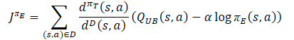
The πе research policy should study the optimistic bias relative to the estimated Q-function values in order to gain experience for effectively correcting false estimates. Therefore, the method authors proposed using an approximate upper bound similar to Optimistic Actor-Critic QUB as a Critic in the objective function. The ultimate goal of the πе policy and a better estimate of the Q-function is to facilitate a more accurate estimate of the gradient for the πт target policy. Therefore, the sampling distribution for the πе loss function should be consistent with the πт behavioral policy. As a consequence, the method authors propose to use the same correction coefficient as for the loss function of the Actor’s target policy.
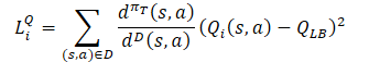
Regarding Critics, the previously discussed approach from Soft Actor-Critic is retained. The lower bound of the Q-function of the target models is used to train them. However, there are a number of studies that prove the efficiency of using the same samples to train Actors and Critics. Therefore, a distribution correction factor was also added to the Critics loss function.
As you can see, the distribution correction coefficient raises the greatest number of questions from everything described above. Let's consider it in detail.
2. Distribution correction
The Distribution Correction Estimation (DICE) algorithm family is designed to solve the issue of the Off-Policy Evaluation (OPE) correction. These methods allow us to train an estimator of the policy value, that is, the normalized expected reward for one step based on the D static retry buffer. DICE receives an unbiased estimator that estimates the distribution correction coefficient.
![]()
To estimate the distribution correction coefficient, the method authors adapted the DICE optimization structure, which can be formulated as a minimax linear distribution program with various regularizations. Directly applying DICE algorithms to off-policy reinforcement learning settings poses significant optimization challenges. Evaluation-free training assumes a fixed goal policy and a static replay buffer with sufficient state-action space coverage, while in RL the goal policy and experience replay buffer change during training. Therefore, the SAC+DICE method authors make several modifications to overcome these difficulties. We will not dive into math now and dwell on these modifications. You can find them in the original article. I will present only the loss functions obtained as a result of the proposed modifications.
![]()
![]()
![]()
Here ζ(s,a) and v(s,a) are models of neural networks, while λ is an adjustable Lagrange coefficient. ζ(s,a) approximates the distribution correction factor. v(s,a) is a sort of critic. In order to stabilize training, we will use the v target model with a soft update of its parameters similar to the Critic.
To optimize all parameters, the authors propose to use the Adam method.
All of the above is generalized into a single SAC+DICE algorithm. As with conventional off-policy reinforcement learning algorithms, we sequentially perform interactions with the environment, following the πе optimistic exploration policy, and save the data to the experience playback buffer. At each training step, the considered algorithm first updates the models and DICE parameters (v, ζ, λ) using SGD with respect to the above loss functions.
Then we calculate the correction ratio of the ζ distribution from the updated model.
Then, using ζ, we train RL to update πт, πе, Q1 and Q2.
At the end of each training step, the Q1, Q2 and v target models are softly updated.
3. Implementation using MQL5
While reading the theoretical part, you might have noticed how the number of trained models and parameters sharply increases. In fact, the number of trained models has increased from 3 to 6. Their interaction becomes more complicated. At the same time, we expect to receive one model of the Actor’s behavioral policy. In order to hide all the routine work from users, we will slightly change our approach and wrap the entire training in a separate class CNet_SAC_DICE. Our new class will be a successor to the base class of CNet neural network models. In the class body, we will declare 5 trainable models and 3 target models. Here we will also declare a number of internal variables. We will look at their functionality during the implementation.
class CNet_SAC_DICE  : protected CNet
  {
protected:
   CNet              cActorExploer;
   CNet              cCritic1;
   CNet              cCritic2;
   CNet              cTargetCritic1;
   CNet              cTargetCritic2;
   CNet              cZeta;
   CNet              cNu;
   CNet              cTargetNu;
   float             fLambda;
   float             fLambda_m;
   float             fLambda_v;
   int               iLatentLayer;
   //---
   float             fLoss1;
   float             fLoss2;
   float             fZeta;
   //---
   vector<float>     GetLogProbability(CBufferFloat *Actions);

public:
   //---
                     CNet_SAC_DICE(void);
                    ~CNet_SAC_DICE(void) {}
   //---
   bool              Create(CArrayObj *actor, CArrayObj *critic, CArrayObj *zeta, CArrayObj *nu, int latent_layer = -1);
   //---
   virtual bool      Study(CArrayFloat *State, CArrayFloat *SecondInput, CBufferFloat *Actions,
                           vector<float> &ActionsLogProbab, CBufferFloat *NextState,
                           CBufferFloat *NextSecondInput, float reward, float discount, float tau);
   virtual void      GetLoss(float &loss1, float &loss2)    {  loss1 = fLoss1; loss2 = fLoss2;  }
   //---
   virtual bool      Save(string file_name, bool common = true);
   bool              Load(string file_name, bool common = true);
  };
Please note that we initially mentioned 6 trainable models, while declaring only 5. Among the announced models, there is no target policy of the Actor. However, the goal of the entire training is precisely to obtain it. As mentioned earlier, our new class is a successor of the base neural network class. This means that it itself is a learning model. Therefore, training the basic Actor policy will be carried out using the parent class.
Also, the new CNet_SAC_DICE class being created will only be used for model training. During operation, creating objects of additional models does not make sense and is an unnecessary consumption of resources. Therefore, we plan to use basic model objects during operation. Due to the above, the new class does not have forward or backward pass methods. All functionality will be implemented in the Study method.
Of course, there are methods for working with the Save and Load files. But first things first.
In the class constructor, we initialize internal variables with initial values. All internal objects are declared statically and are not subject to initialization. Accordingly, we do not need to clear memory in the destructor, which allows us to leave the destructor empty.
CNet_SAC_DICE::CNet_SAC_DICE(void)  :  fLambda(1.0e-5f),
                                       fLambda_m(0),
                                       fLambda_v(0),
                                       fLoss1(0),
                                       fLoss2(0),
                                       fZeta(0)
  {
  }
Full initialization of models is carried out in the Create method. In the method parameters, we will pass the dynamic arrays of descriptions of the all used models' architecture and the ID of the Actor’s latent layer with a compressed representation of the analyzed state of the environment.
In the method body, we will first create the Actor models. The optimistic model is created in the cActorExploer object. The target model is created in the body of our class using the tools that have been inherited.
bool CNet_SAC_DICE::Create(CArrayObj *actor, CArrayObj *critic, CArrayObj *zeta, CArrayObj *nu, int latent_layer)
  {
   ResetLastError();
//---
   if(!cActorExploer.Create(actor) || !CNet::Create(actor))
     {
      PrintFormat("Error of create Actor: %d", GetLastError());
      return false;
     }
//---
   if(!opencl)
     {
      Print("Don't opened OpenCL context");
      return false;
     }
We immediately check the created OpenCL context pointer.
Next, we create trainable models of both Critics.
   if(!cCritic1.Create(critic) || !cCritic2.Create(critic))
     {
      PrintFormat("Error of create Critic: %d", GetLastError());
      return false;
     }
They are followed by the block DICE objects and target models.
   if(!cZeta.Create(zeta) || !cNu.Create(nu))
     {
      PrintFormat("Error of create function nets: %d", GetLastError());
      return false;
     }
//---
   if(!cTargetCritic1.Create(critic) || !cTargetCritic2.Create(critic) ||
      !cTargetNu.Create(nu))
     {
      PrintFormat("Error of create target models: %d", GetLastError());
      return false;
     }
After successfully creating all the models, we will pass them to a single OpenCL context.
   cActorExploer.SetOpenCL(opencl);
   cCritic1.SetOpenCL(opencl);
   cCritic2.SetOpenCL(opencl);
   cZeta.SetOpenCL(opencl);
   cNu.SetOpenCL(opencl);
   cTargetCritic1.SetOpenCL(opencl);
   cTargetCritic2.SetOpenCL(opencl);
   cTargetNu.SetOpenCL(opencl);
And copy the model parameters to their target copies. Also, we should not forget to control the execution of operations at every step.
   if(!cTargetCritic1.WeightsUpdate(GetPointer(cCritic1), 1.0) ||
      !cTargetCritic2.WeightsUpdate(GetPointer(cCritic2), 1.0) ||
      !cTargetNu.WeightsUpdate(GetPointer(cNu), 1.0))
     {
      PrintFormat("Error of update target models: %d", GetLastError());
      return false;
     }
After successfully creating all the necessary objects, we will transfer the data to internal variables and terminate the method.
   fLambda = 1.0e-5f;
   fLambda_m = 0;
   fLambda_v = 0;
   fZeta = 0;
   iLatentLayer = latent_layer;
//---
   return true;
  }
After initializing the internal objects of the class, we proceed to work on the CNet_SAC_DICE::Study model training method. In the parameters of this class, we receive all the information necessary for one step of training the model. Here are the current and future states of the environment. In this case, each state is described in two data buffers: historical data and balance state. Here you will also see the action buffer and reward variable. There are also variables for discount rates and soft updating of target models. For the first time, we add a vector of logarithms of the probability of the original policy (used in collecting examples).
bool CNet_SAC_DICE::Study(CArrayFloat *State,
                          CArrayFloat *SecondInput,
                          CBufferFloat *Actions,
                          vector<float> &ActionsLogProbab,
                          CBufferFloat *NextState,
                          CBufferFloat *NextSecondInput,
                          float reward,
                          float discount,
                          float tau)
  {
//---
   if(!Actions || Actions.Total()!=ActionsLogProbab.Size())
      return false;
In the body of the method, we first arrange a small control block where we check the relevance of the pointer to the action buffer and the correspondence of its size and the size of the probability logarithm vector. We do not check pointers to other buffers, since their control is implemented in the called methods.
After successfully passing the control block, we carry out subsequent state assessments by the target models taking into account the current policy. To do this, we first implement a direct pass of our conservative Actor policy. We use it to preprocess raw data describing the current state and predict the action vector from this state. We pass the obtained data to two target models of Critics and the v model from the DICE block.
   if(!CNet::feedForward(NextState, 1, false, NextSecondInput))
      return false;
   if(!cTargetCritic1.feedForward(GetPointer(this), iLatentLayer, GetPointer(this), layers.Total() - 1) ||
      !cTargetCritic2.feedForward(GetPointer(this), iLatentLayer, GetPointer(this), layers.Total() - 1))
      return false;
//---
   if(!cTargetNu.feedForward(GetPointer(this), iLatentLayer, GetPointer(this), layers.Total() - 1))
      return false;
The next step is to prepare the current state data. As with the subsequent state, we use the current conservative Actor model to preprocess the description of the current state.
   if(!CNet::feedForward(State, 1, false, SecondInput))
      return false;
   CBufferFloat *output = ((CNeuronBaseOCL*)((CLayer*)layers.At(layers.Total() - 1)).At(0)).getOutput();
   output.AssignArray(Actions);
   output.BufferWrite();
Here we perform a small trick replacing the results of a forward pass. Instead of the obtained actions of the current Actor policy, we will save the action tensor from the experience reproduction buffer into the results buffer of the last neural layer. The purpose of this operation is to maintain the correspondence between the action and the reward from the environment. We are aware that other actions were most likely formed during the forward pass. But our CNeuronSoftActorCritic neural layer studies the distribution of actions and their probabilities in the depths of its internal objects. During the reverse pass, quantiles and probabilities will be determined corresponding to actions from the experience playback buffer. In this case, the unbiased gradient will pass precisely to these quantiles, which will allow the Actor model to be trained more accurately and without distortion.
After preparing the current environmental state data, we can perform a forward pass through the block DICE models. Remember to control the execution of operations.
   if(!cNu.feedForward(GetPointer(this), iLatentLayer, GetPointer(this)))
      return false;
   if(!cZeta.feedForward(GetPointer(this), iLatentLayer, GetPointer(this)))
      return false;
In accordance with the SAC+DICE algorithm, we first update the models and parameters of the block DICE. But before updating the parameters, we need to calculate the values of the loss functions for v, ζ, λ.
Note that to obtain the value of the loss functions, we need a target value of the state-action probability ratio in the current conservative policy and in interaction with the environment during the collection of the example base. Here it should be said that the historical data describing the state of the environment do not depend on the Actor policies. Moreover, we perceive the current state as the starting point for making a decision and building a subsequent trajectory of an action. Consequently, the probability of the initial state is perceived as equal to 1, because we are in it.
During the policy training, only the probabilistic distribution of actions changes in accordance with the learned strategy. Therefore, our target value will be the ratio of the probabilities of actions in the two policies. During the operations, we will use the difference of the probability logarithms instead of the probability ratio. In this case, instead of multiplying the probabilities of all actions, we will use the sum of their logarithms and restore the value through an exponent.
   vector<float> nu, next_nu, zeta, ones;
   cNu.getResults(nu);
   cTargetNu.getResults(next_nu);
   cZeta.getResults(zeta);
   ones = vector<float>::Ones(zeta.Size());
   vector<float> log_prob = GetLogProbability(output);
   float policy_ratio = MathExp((log_prob - ActionsLogProbab).Sum());
   vector<float> bellman_residuals = next_nu * discount * policy_ratio - nu + policy_ratio * reward;
   vector<float> zeta_loss = zeta * (MathAbs(bellman_residuals) - fLambda) * (-1) + MathPow(zeta, 2.0f) / 2;
   vector<float> nu_loss = zeta * MathAbs(bellman_residuals) + MathPow(nu, 2.0f) / 2.0f;
   float lambda_los = fLambda * (ones - zeta).Sum();
After determining the loss function values, we will define the error gradients and update the parameters. First, we update the Lagrange coefficient values. During the parameter adjustment, we use the Adam method algorithm.
//--- update lambda
   float grad_lambda = (ones - zeta).Sum() * (-lambda_los);
   fLambda_m = b1 * fLambda_m + (1 - b1) * grad_lambda;
   fLambda_v = b2 * fLambda_v + (1 - b2) * MathPow(grad_lambda, 2);
   fLambda += lr * fLambda_m / (fLambda_v != 0.0f ? MathSqrt(fLambda_v) : 1.0f);
Next we need to update the v, ζ models' parameters. Keep in mind that we have defined the values of the loss functions, not the target values. Moreover, the loss function for each model is individual and very different from those previously used by us. Currently, we will not fit the operations to the basic loss function of our model. Instead, we will immediately calculate the error gradient. Let's transfer the resulting value to the appropriate model buffer and propagate the error gradient across the model parameters.
First, update the v model parameters.
//---
   CBufferFloat temp;
   temp.BufferInit(MathMax(Actions.Total(), SecondInput.Total()), 0);
   temp.BufferCreate(opencl);
//--- update nu
   int last_layer = cNu.layers.Total() - 1;
   CLayer *layer = cNu.layers.At(last_layer);
   if(!layer)
      return false;
   CNeuronBaseOCL *neuron = layer.At(0);
   if(!neuron)
      return false;
   CBufferFloat *buffer = neuron.getGradient();
   if(!buffer)
      return false;
   vector<float> nu_grad = nu_loss * (zeta * bellman_residuals / MathAbs(bellman_residuals) + nu);
   if(!buffer.AssignArray(nu_grad) || !buffer.BufferWrite())
      return false;
   if(!cNu.backPropGradient(output, GetPointer(temp)))
      return false;
Then perform similar operations for the ζ model.
//--- update zeta
   last_layer = cZeta.layers.Total() - 1;
   layer = cZeta.layers.At(last_layer);
   if(!layer)
      return false;
   neuron = layer.At(0);
   if(!neuron)
      return false;
   buffer = neuron.getGradient();
   if(!buffer)
      return false;
   vector<float> zeta_grad = zeta_loss * (zeta - MathAbs(bellman_residuals) + fLambda) * (-1);
   if(!buffer.AssignArray(zeta_grad) || !buffer.BufferWrite())
      return false;
   if(!cZeta.backPropGradient(output, GetPointer(temp)))
      return false;
At this point, we have updated the DICE block parameters and are moving directly to the reinforcement learning procedure. First, carry out a direct passage of both Critics. In this case, we do not perform a direct pass of the Actor, since we have already performed this operation when updating the parameters of the DICE objects of the block.
//--- feed forward critics
   if(!cCritic1.feedForward(GetPointer(this), iLatentLayer, output) ||
      !cCritic2.feedForward(GetPointer(this), iLatentLayer, output))
      return false;
Next, as with updating DICE parameters, we will determine the values of the loss functions. But first, let's do a little preparatory work. To increase the stability of model training, we normalize the distribution correction coefficient and calculate the reference value predicted by the target critic models taking into account the current Actor policy.
   vector<float> result;
   if(fZeta == 0)
      fZeta = MathAbs(zeta[0]);
   else
      fZeta = 0.9f * fZeta + 0.1f * MathAbs(zeta[0]);
   zeta[0] = MathPow(MathAbs(zeta[0]), 1.0f / 3.0f) / (10.0f * MathPow(fZeta, 1.0f / 3.0f));
   cTargetCritic1.getResults(result);
   float target = result[0];
   cTargetCritic2.getResults(result);
   target = reward + discount * (MathMin(result[0], target) - LogProbMultiplier * log_prob.Sum());
Despite the presence of a target value, we cannot implement the basic method of back-passing the critics' models, since the use of a distribution correction coefficient does not fit into it. Therefore, we use the above-developed technique with the calculation of the error gradient and its direct transfer to the buffer of the neural layer of the results followed by the distribution of gradients over the model.
//--- update critic1
   cCritic1.getResults(result);
   float loss = zeta[0] * MathPow(result[0] - target, 2.0f);
   if(fLoss1 == 0)
      fLoss1 = MathSqrt(loss);
   else
      fLoss1 = MathSqrt(0.999f * MathPow(fLoss1, 2.0f) + 0.001f * loss);
   float grad = loss * 2 * zeta[0] * (target - result[0]);
   last_layer = cCritic1.layers.Total() - 1;
   layer = cCritic1.layers.At(last_layer);
   if(!layer)
      return false;
   neuron = layer.At(0);
   if(!neuron)
      return false;
   buffer = neuron.getGradient();
   if(!buffer)
      return false;
   if(!buffer.Update(0, grad) || !buffer.BufferWrite())
      return false;
   if(!cCritic1.backPropGradient(output, GetPointer(temp)) ||
      !backPropGradient(SecondInput, GetPointer(temp), iLatentLayer))
      return false;
At the same time, we calculate the average error of the model, which we will show to the user for visual control of the model training process.
Repeat the operations for the second critic.
//--- update critic2
   cCritic2.getResults(result);
   loss = zeta[0] * MathPow(result[0] - target, 2.0f);
   if(fLoss2 == 0)
      fLoss2 = MathSqrt(loss);
   else
      fLoss2 = MathSqrt(0.999f * MathPow(fLoss1, 2.0f) + 0.001f * loss);
   grad = loss * 2 * zeta[0] * (target - result[0]);
   last_layer = cCritic2.layers.Total() - 1;
   layer = cCritic2.layers.At(last_layer);
   if(!layer)
      return false;
   neuron = layer.At(0);
   if(!neuron)
      return false;
   buffer = neuron.getGradient();
   if(!buffer)
      return false;
   if(!buffer.Update(0, grad) || !buffer.BufferWrite())
      return false;
   if(!cCritic2.backPropGradient(output, GetPointer(temp)) ||
      !backPropGradient(SecondInput, GetPointer(temp), iLatentLayer))
      return false;
After updating the Critics' parameters, we move on to updating the Actors' policies. We will update the Conservative Actor's policy first. Here we calculate the target value taking into account the lower bound of the Q-function values and the current probability distribution of the actions. We will correct the resulting value by the distribution correction coefficient and draw the error gradient through the Critic's model. First, we will disable the training mode of the critic.
//--- update policy
   cCritic1.getResults(result);
   float mean = result[0];
   float var = result[0];
   cCritic2.getResults(result);
   mean += result[0];
   var -= result[0];
   mean /= 2.0f;
   var = MathAbs(var) / 2.0f;
   target = zeta[0] * (mean - 2.5f * var + discount * log_prob.Sum() * LogProbMultiplier) + result[0];
   CBufferFloat bTarget;
   bTarget.Add(target);
   cCritic2.TrainMode(false);
   if(!cCritic2.backProp(GetPointer(bTarget), GetPointer(this)) ||
      !backPropGradient(SecondInput, GetPointer(temp)))
     {
      cCritic2.TrainMode(true);
      return false;
     }
Before updating the parameters of the optimistic research policy of the Actor, we perform a forward pass through the specified model and replace the values of the result buffer (as we previously did for the pessimistic model).
Then we recalculate the target value taking into account the optimism coefficient and distribute the error gradient through the critic model.
//--- update exploration policy
   if(!cActorExploer.feedForward(State, 1, false, SecondInput))
     {
      cCritic2.TrainMode(true);
      return false;
     }
   output = ((CNeuronBaseOCL*)((CLayer*)cActorExploer.layers.At(layers.Total() - 1)).At(0)).getOutput();
   output.AssignArray(Actions);
   output.BufferWrite();
   cActorExploer.GetLogProbs(log_prob);
   target = zeta[0] * (mean + 2.0f * var + discount * log_prob.Sum() * LogProbMultiplier) + result[0];
   bTarget.Update(0, target);
   if(!cCritic2.backProp(GetPointer(bTarget), GetPointer(cActorExploer)) ||
      !cActorExploer.backPropGradient(SecondInput, GetPointer(temp)))
     {
      cCritic2.TrainMode(true);
      return false;
     }
   cCritic2.TrainMode(true);
After completing the operations, we turn on the critic training mode and update the parameters of the target models.
   if(!cTargetCritic1.WeightsUpdate(GetPointer(cCritic1), tau) ||
      !cTargetCritic2.WeightsUpdate(GetPointer(cCritic2), tau) ||
      !cTargetNu.WeightsUpdate(GetPointer(cNu), tau))
     {
      PrintFormat("Error of update target models: %d", GetLastError());
      return false;
     }
//---
   return true;
  }
We have completed the work on the model training method. Now it is time to move on to building the methods for working with files. First we create a method for saving the models. Unlike previously discussed similar methods, we will not save all the data in one file. In contrast, each trained model will receive a separate file. This will allow us to use each individual model independently of the others.
In the parameters, the data saving method CNet_SAC_DICE::Save will receive the common file name (without extension) and the save flag in the shared terminal folder. In the method body, we immediately check the presence of the file name in the resulting text variable.
bool CNet_SAC_DICE::Save(string file_name, bool common = true)
  {
   if(file_name == NULL)
      return false;
Next, we create a file with the given name and ".set" extension. The values of internal variables will be saved into it.
   int handle = FileOpen(file_name + ".set", (common ? FILE_COMMON : 0) | FILE_BIN | FILE_WRITE);
   if(handle == INVALID_HANDLE)
      return false;
   if(FileWriteFloat(handle, fLambda) < sizeof(fLambda) ||
      FileWriteFloat(handle, fLambda_m) < sizeof(fLambda_m) ||
      FileWriteFloat(handle, fLambda_v) < sizeof(fLambda_v) ||
      FileWriteInteger(handle, iLatentLayer) < sizeof(iLatentLayer))
      return false;
   FileFlush(handle);
   FileClose(handle);
After that, we call the methods for saving models one by one and control the process of performing operations. Here it is worth paying attention to the specified file names. An Actor with a conservative policy receives the file name suffix of "Act.nnw" (as we previously specified for Actors). The optimistic Actor model receives a file with the ActExp.nnw suffix. In addition, we only store the target models of Critics and v models. The corresponding trained models are not saved.
   if(!CNet::Save(file_name + "Act.nnw", 0, 0, 0, TimeCurrent(), common))
      return false;
//---
   if(!cActorExploer.Save(file_name + "ActExp.nnw", 0, 0, 0, TimeCurrent(), common))
      return false;
//---
   if(!cTargetCritic1.Save(file_name + "Crt1.nnw", fLoss1, 0, 0, TimeCurrent(), common))
      return false;
//---
   if(!cTargetCritic2.Save(file_name + "Crt2.nnw", fLoss2, 0, 0, TimeCurrent(), common))
      return false;
//---
   if(!cZeta.Save(file_name + "Zeta.nnw", 0, 0, 0, TimeCurrent(), common))
      return false;
//---
   if(!cTargetNu.Save(file_name + "Nu.nnw", 0, 0, 0, TimeCurrent(), common))
      return false;
//---
   return true;
  }
In the data loading method, we repeat the operations in strict accordance with the order, in which the data was set. In this case, the trained and target models are loaded from the same corresponding files.
bool CNet_SAC_DICE::Load(string file_name, bool common = true)
  {
   if(file_name == NULL)
      return false;
//---
   int handle = FileOpen(file_name + ".set", (common ? FILE_COMMON : 0) | FILE_BIN | FILE_READ);
   if(handle == INVALID_HANDLE)
      return false;
   if(FileIsEnding(handle))
      return false;
   fLambda = FileReadFloat(handle);
   if(FileIsEnding(handle))
      return false;
   fLambda_m = FileReadFloat(handle);
   if(FileIsEnding(handle))
      return false;
   fLambda_v =   FileReadFloat(handle);
   if(FileIsEnding(handle))
      return false;
   iLatentLayer =  FileReadInteger(handle);;
   FileClose(handle);
//---
   float temp;
   datetime dt;
   if(!CNet::Load(file_name + "Act.nnw", temp, temp, temp, dt, common))
      return false;
//---
   if(!cActorExploer.Load(file_name + "ActExp.nnw", temp, temp, temp, dt, common))
      return false;
//---
   if(!cCritic1.Load(file_name + "Crt1.nnw", fLoss1, temp, temp, dt, common) ||
      !cTargetCritic1.Load(file_name + "Crt1.nnw", temp, temp, temp, dt, common))
      return false;
//---
   if(!cCritic2.Load(file_name + "Crt2.nnw", fLoss2, temp, temp, dt, common) ||
      !cTargetCritic2.Load(file_name + "Crt2.nnw", temp, temp, temp, dt, common))
      return false;
//---
   if(!cZeta.Load(file_name + "Zeta.nnw", temp, temp, temp, dt, common))
      return false;
//---
   if(!cNu.Load(file_name + "Nu.nnw", temp, temp, temp, dt, common) ||
      !cTargetNu.Load(file_name + "Nu.nnw", temp, temp, temp, dt, common))
      return false;
After loading these models, we transfer them into a single OpenCL context.
   cActorExploer.SetOpenCL(opencl);
   cCritic1.SetOpenCL(opencl);
   cCritic2.SetOpenCL(opencl);
   cZeta.SetOpenCL(opencl);
   cNu.SetOpenCL(opencl);
   cTargetCritic1.SetOpenCL(opencl);
   cTargetCritic2.SetOpenCL(opencl);
   cTargetNu.SetOpenCL(opencl);
//---
   return true;
  }
This completes our work on the CNet_SAC_DICE class. You can find a complete code of all its methods in the attachment. As you might remember, the parameters of the training method discussed above indicate a vector of logarithms of action probabilities. But we have not saved such data to the experience playback buffer before. Therefore, now we need to add the corresponding array to the SState state-action description structure presented in the file "..\SAC&DICE\Trajectory.mqh". The size of the array is equal to the number of actions.
struct SState
  {
   float             state[HistoryBars * BarDescr];
   float             account[AccountDescr - 4];
   float             action[NActions];
   float             log_prob[NActions];
   //---
                     SState(void);
   //---
   bool              Save(int file_handle);
   bool              Load(int file_handle);
   //--- overloading
   void              operator=(const SState &obj)
     {
      ArrayCopy(state, obj.state);
      ArrayCopy(account, obj.account);
      ArrayCopy(action, obj.action);
      ArrayCopy(log_prob, obj.log_prob);
     }
  };
Do not forget to add the array to the algorithm of methods for copying structure and working with files. The full structure code can be found in the attachment.
Let's move on to creating and training models. Regarding the model architecture, it was transferred from the article, describing the Soft Actor-Critic method, without changes. At the same time, we did not create separate architectures for v and ζ models. We used the critic architecture for them.
While training the model, we use three EAs as before:
- Research — collecting examples database
- Study — model training
- Test — checking obtained results.
When collecting data for the example database in the Research EA, we use the optimistic Actor policy (the file with the "ActExp.nnw" suffix). However, in order to test the trained model, we will use a conservative model (the file with the "Act.nnw" suffix). We should pay attention to this when loading models in the corresponding files. In addition, when collecting data into the experience playback buffer, do not forget to add the loading of the logarithm of the action distribution probabilities. The full EAs' code can be found in the attachment.
The Study training EA has undergone maximum changes. This is not surprising. We transferred a huge part of its functionality to the Study training method of the CNet_SAC_DICE class.
We start by changing the library containing our model.
#include "Net_SAC_DICE.mqh"
In the global variables block, we declare only one model of the newly created CNet_SAC_DICE class. At the same time, we increase the number of data buffers. This is due to the fact that previously we could use one buffer for two states at different stages of training. Now we will have to simultaneously transmit information about two subsequent states to the model.
STrajectory          Buffer[];
CNet_SAC_DICE        Net;
//---
float                dError;
datetime             dtStudied;
//---
CBufferFloat         bState;
CBufferFloat         bAccount;
CBufferFloat         bActions;
CBufferFloat         bNextState;
CBufferFloat         bNextAccount;
As before, in the EA initialization method, we first load the experience playback buffer for training models.
int OnInit()
  {
//---
   ResetLastError();
   if(!LoadTotalBase())
     {
      PrintFormat("Error of load study data: %d", GetLastError());
      return INIT_FAILED;
     }
After that, we load a single model. If the model has not yet been created, then we form arrays of descriptions of the model architecture and create only one model, passing all the architecture descriptions to it. We check the operations result only once.
As mentioned above, we provide a description of the critic's architecture for DICE block models. But other options are also possible. When creating your own models for this block, pay attention to the use of the Actor model as a block of primary processing of source data. This is exactly how we built the entire model training algorithm. We need to either follow it when creating model architectures, or make appropriate changes to the method algorithm.
//--- load models
   if(!Net.Load(FileName, true))
     {
      CArrayObj *actor = new CArrayObj();
      CArrayObj *critic = new CArrayObj();
      if(!CreateDescriptions(actor, critic))
        {
         delete actor;
         delete critic;
         return INIT_FAILED;
        }
      if(!Net.Create(actor, critic, critic, critic, LatentLayer))
        {
         delete actor;
         delete critic;
         return INIT_FAILED;
        }
      delete actor;
      delete critic;
     }
When I say "only a single model", I might not be completely accurate. During the training process, we create 6 updated models and 3 target ones. All models are created inside our new class and are hidden from the user. At the top level, we only work with one class.
At the end of the EA initialization method, we generate a model training event.
   if(!EventChartCustom(ChartID(), 1, 0, 0, "Init"))
     {
      PrintFormat("Error of create study event: %d", GetLastError());
      return INIT_FAILED;
     }
//---
   return(INIT_SUCCEEDED);
  }
After successfully completing all operations, we complete the EA initialization procedure.
The next step is to move on to working on the procedure for directly training Train models.
As before, we arrange a training cycle in the body of this function according to the number of iterations specified in the EA external parameters.
void Train(void)
  {
   int total_tr = ArraySize(Buffer);
   uint ticks = GetTickCount();
//---
   for(int iter = 0; (iter < Iterations && !IsStopped()); iter ++)
     {
      int tr = (int)((MathRand() / 32767.0) * (total_tr - 1));
      int i = (int)((MathRand() * MathRand() / MathPow(32767, 2)) * (Buffer[tr].Total - 2));
      if(i<0)
        {
         iter--;
         continue;
        }
Inside the loop, we sample the trajectory and individual step for the current iteration of model training.
Next, we will carry out the preparatory work and collect the necessary data into the previously declared data buffers. First, we will buffer the historical data describing the subsequent state of the environment.
      //--- Target
      bNextState.AssignArray(Buffer[tr].States[i + 1].state);
      float PrevBalance = Buffer[tr].States[i].account[0];
      float PrevEquity = Buffer[tr].States[i].account[1];
      if(PrevBalance==0)
        {
         iter--;
         continue;
        }
      bNextAccount.Clear();
      bNextAccount.Add((Buffer[tr].States[i + 1].account[0] - PrevBalance) / PrevBalance);
      bNextAccount.Add(Buffer[tr].States[i + 1].account[1] / PrevBalance);
      bNextAccount.Add((Buffer[tr].States[i + 1].account[1] - PrevEquity) / PrevEquity);
      bNextAccount.Add(Buffer[tr].States[i + 1].account[2]);
      bNextAccount.Add(Buffer[tr].States[i + 1].account[3]);
      bNextAccount.Add(Buffer[tr].States[i + 1].account[4] / PrevBalance);
      bNextAccount.Add(Buffer[tr].States[i + 1].account[5] / PrevBalance);
      bNextAccount.Add(Buffer[tr].States[i + 1].account[6] / PrevBalance);
      double x = (double)Buffer[tr].States[i + 1].account[7] / (double)(D'2024.01.01' - D'2023.01.01');
      bNextAccount.Add((float)MathSin(x != 0 ? 2.0 * M_PI * x : 0));
      x = (double)Buffer[tr].States[i + 1].account[7] / (double)PeriodSeconds(PERIOD_MN1);
      bNextAccount.Add((float)MathCos(x != 0 ? 2.0 * M_PI * x : 0));
      x = (double)Buffer[tr].States[i + 1].account[7] / (double)PeriodSeconds(PERIOD_W1);
      bNextAccount.Add((float)MathSin(x != 0 ? 2.0 * M_PI * x : 0));
      x = (double)Buffer[tr].States[i + 1].account[7] / (double)PeriodSeconds(PERIOD_D1);
      bNextAccount.Add((float)MathSin(x != 0 ? 2.0 * M_PI * x : 0));
In another buffer, we will create a description of the account status and add timestamps.
In a similar way, we will prepare buffers describing the analyzed state of the environment.
      bState.AssignArray(Buffer[tr].States[i].state);
      PrevBalance = Buffer[tr].States[MathMax(i - 1, 0)].account[0];
      PrevEquity = Buffer[tr].States[MathMax(i - 1, 0)].account[1];
      bAccount.Clear();
      bAccount.Add((Buffer[tr].States[i].account[0] - PrevBalance) / PrevBalance);
      bAccount.Add(Buffer[tr].States[i].account[1] / PrevBalance);
      bAccount.Add((Buffer[tr].States[i].account[1] - PrevEquity) / PrevEquity);
      bAccount.Add(Buffer[tr].States[i].account[2]);
      bAccount.Add(Buffer[tr].States[i].account[3]);
      bAccount.Add(Buffer[tr].States[i].account[4] / PrevBalance);
      bAccount.Add(Buffer[tr].States[i].account[5] / PrevBalance);
      bAccount.Add(Buffer[tr].States[i].account[6] / PrevBalance);
      x = (double)Buffer[tr].States[i].account[7] / (double)(D'2024.01.01' - D'2023.01.01');
      bAccount.Add((float)MathSin(x != 0 ? 2.0 * M_PI * x : 0));
      x = (double)Buffer[tr].States[i].account[7] / (double)PeriodSeconds(PERIOD_MN1);
      bAccount.Add((float)MathCos(x != 0 ? 2.0 * M_PI * x : 0));
      x = (double)Buffer[tr].States[i].account[7] / (double)PeriodSeconds(PERIOD_W1);
      bAccount.Add((float)MathSin(x != 0 ? 2.0 * M_PI * x : 0));
      x = (double)Buffer[tr].States[i].account[7] / (double)PeriodSeconds(PERIOD_D1);
      bAccount.Add((float)MathSin(x != 0 ? 2.0 * M_PI * x : 0));
Then we will move the completed actions to the buffer. The probability logarithm will be loaded into the vector.
      bActions.AssignArray(Buffer[tr].States[i].action);
      vector<float> log_prob;
      log_prob.Assign(Buffer[tr].States[i].log_prob);
At this stage, we complete the preparatory work. All the data necessary for one training iteration has already been collected in the data buffers. We call the CNet_SAC_DICE::Study training method of our model passing the necessary data in the parameters.
      if(!Net.Study(GetPointer(bState), GetPointer(bAccount), GetPointer(bActions), log_prob,
                    GetPointer(bNextState), GetPointer(bNextAccount),
                    Buffer[tr].Revards[i] - DiscFactor * Buffer[tr].Revards[i + 1], DiscFactor, Tau))
        {
         PrintFormat("%s -> %d", __FUNCTION__, __LINE__);
         break;
        }
Please note that in the experience replay buffer we stored the rewards as a cumulative total. Now we transfer the net reward for one individual step to the model training method. Missing data will be predicted by target models.
We implemented all model training operations to the training method of our class. Now we just need to check the result of the method operations. Then we will inform the user about the the model training process.
      if(GetTickCount() - ticks > 500)
        {
         float loss1, loss2;
         Net.GetLoss(loss1, loss2);
         string str = StringFormat("%-15s %5.2f%% -> Error %15.8f\n", "Critic1",
                                    iter * 100.0 / (double)(Iterations), loss1);
         str += StringFormat("%-15s %5.2f%% -> Error %15.8f\n", "Critic2",
                                    iter * 100.0 / (double)(Iterations), loss2);
         Comment(str);
         ticks = GetTickCount();
        }
     }
After completing the loop iterations, we clear the comment field and initiate the EA shutdown process.
   Comment("");
//---
   float loss1, loss2;
   Net.GetLoss(loss1, loss2);
   PrintFormat("%s -> %d -> %-15s %10.7f", __FUNCTION__, __LINE__, "Critic1", loss1);
   PrintFormat("%s -> %d -> %-15s %10.7f", __FUNCTION__, __LINE__, "Critic2", loss2);
   ExpertRemove();
//---
  }
As we can see, placing model training operations into a separate class method allows us to significantly reduce code and labor costs on the side of the main program. At the same time, this approach reduces the flexibility of the model training and the user's ability to adjust it. Both approaches have their positive and negative sides. The choice of a specific approach depends on the task at hand and personal preferences.
The full code of the EA and all programs used in the article is available in the attachment.
4. Test
The model was trained on historical data of EURUSD H1 within January - May 2023. The indicator parameters and all hyperparameters were set to their default values. During the training process, a model was obtained that was capable of generating profit on the training set.


Over the 5-month training period, the model was able to earn 15% of profit. 314 positions were opened, 45.8% of which were closed with a profit. The maximum profitable trade exceeds the maximum loss almost 2 times. Moreover, the average profitable trade is 1/3 higher than the average loss. It was this ratio of profits and losses that allowed us to obtain a profit factor of 1.13.
As usual, we are much more interested in the efficiency of the model on new data. The generalization ability and performance of the model on unfamiliar data was tested in the strategy tester on historical data for June 2023. As we can see, the testing period immediately follows the training set. This ensures maximum homogeneity of the training and test samples. The test results are presented below.

The presented chart shows a drawdown area in the first ten days of the month. But then it is followed by a period of profitability, which lasts until the end of the month. As a result, the EA received a profit of 7.7% over the course of the month with a maximum drawdown in Equity of 5.46%. In terms of the balance, the drawdown was even smaller and did not exceed 4.87%.

The table of test results shows that during the test the EA performed trades in both directions. A total of 48 positions were opened. 54.17% of them were closed with a profit. The maximum profitable trade is more than 3 times higher than the maximum losing one. The average profitable trade is half as much as the average losing trade. In quantitative terms, on average, for every 3 profitable trades there are 2 unprofitable ones. All this gave a profit factor of 1.74 and a recovery factor of 1.41.
Conclusion
The article considered another algorithm from the Actor-Critic family - the SAC+DICE algorithm based on two main directions of modification of the Soft Actor-Critic algorithm. The use of an optimistic model of environmental research allows us to expand the area of environmental research. The research is carried out in the direction of increasing the profitability of the general policy. Of course, this leads to a break in the distributions of environmental research policies and learning conservative policies. To obtain an unbiased estimate of gradients, we used a modified DICE approach and introduced a trainable distribution correction coefficient. All this makes it possible to increase the efficiency of model training, which was confirmed in the practical part of our article.
We implemented the proposed algorithm using MQL5. During this implementation, an approach was demonstrated to move the model training process into a separate class method. This allows us to significantly reduce work on the side of the main program and simplify the usage.
We trained and tested the trained model on new data. Test results demonstrated the efficiency of our implementation. The trained model was able to transfer the experience gained to new data. During the test, the EA made a profit.
However, all the programs presented only demonstrate the possibility of using the technology. They are not ready for use in real financial markets. The EAs need to be refined and additionally tested before being launched on a real market.
Links
Programs used in the article
| # | Name | Type | Description |
|---|---|---|---|
| 1 | Research.mq5 | Expert Advisor | Example collection EA |
| 2 | Study.mq5 | Expert Advisor | Agent training EA |
| 3 | Test.mq5 | Expert Advisor | Model testing EA |
| 4 | Trajectory.mqh | Class library | System state description structure |
| 5 | Net_SAC_DICE.mqh | Class library | Model class |
| 6 | NeuroNet.mqh | Class library | A library of classes for creating a neural network |
| 7 | NeuroNet.cl | Code Base | OpenCL program code library |
Translated from Russian by MetaQuotes Ltd.
Original article: https://www.mql5.com/ru/articles/13055
- Free trading apps
- Over 8,000 signals for copying
- Economic news for exploring financial markets
You agree to website policy and terms of use
Dmitry, why does this network open all trades with exactly 1 lot, when training on all tests, and does not try to change the lot? It doesn't try to put fractional lots and doesn't want to put more than 1 lot either. EURUSD instrument. Training parameters are the same as yours.
On the last Actor layer we use sigmoid as an activation function, which limits the values in the range [0,1]. For TP and SL, we use a multiplier to adjust the values. The lot size is not adjusted. Therefore, 1 lot is the maximum possible value.
In the last Actor layer, we use sigmoid as the activation function, which limits the values to the range [0,1]. For TP and SL we use a multiplier to adjust the values. The lot size is not adjusted. Therefore, 1 lot is the maximum possible value.
Understood, Thank you.