Neural networks made easy (Part 51): Behavior-Guided Actor-Critic (BAC)

Introduction

The last two articles were devoted to the Soft Actor-Critic algorithm. As you remember, the algorithm is used to train stochastic models in a continuous action space. The main feature of this method is the introduction of an entropy component into the reward function, which allows us to adjust the balance between environmental exploration and model operation. At the same time, this approach imposes some restrictions on the trained models. Using entropy requires some idea of the probability of taking actions, which is quite difficult to directly calculate for a continuous space of actions.

We used a quantile distribution approach. Here we add the adjustment of the hyperparameters of the quantile distribution. The very approach of using the quantile distribution moves us a little away from the continuous action space. After all, every time we selected an action, we selected a quantile from the learned probability distribution and used its average value as the action. With a sufficiently large number of quantiles and a sufficiently small range of possible values, we approach a continuous action space. But this leads to a growing complexity of the model and an increase in the costs of its training and operation. Besides, this imposes restrictions on the architecture of trained models.

In this article, we will talk about an alternative approach, Behavior-Guided Actor-Critic (BAC), which was introduced in April 2021.

1. Algorithm construction features

First, let's talk about the need to study the environment in general. I think everyone agrees that this process is necessary. But for what exactly and at what stage?

Let's start with a simple example. Suppose that we find ourselves in a room with three identical doors and we need to get into the street. What shall we do? We open the doors one by one until we find the one we need. When we enter the same room again, we will no longer open all the doors to get outside, but instead we will immediately head to the already known exit. If we have a different task, then some options are possible. We can again open all the doors, except for the exit we already know, and look for the right one. Or we can first remember which doors we opened earlier when looking for a way out and whether the one we need was among them. If we remember the right door, we head towards it. Otherwise, we check the doors we have not tried before.

Conclusion: We need to study the environment in an unfamiliar situation to choose the right action. After finding the required route, additional exploration of the environment can only get in the way.

However, when the task changes in a known state, we may need to additionally study the environment. This may include searching for a more optimal route. In the example above, this may happen if we needed to go through several more rooms or we found ourselves at the wrong side of the building.

Therefore, we need an algorithm that allows us to enhance environmental exploration in unexplored states and minimize it in previously explored states.

The entropy regularization used in Soft Actor-Critic can meet this requirement, but only with a number of conditions. The entropy of an action is high when the action probability is low. Indeed, the state we enter after a low-probability action is likely poorly understood. The entropy regularization pushes us to repeat it in order to better study subsequent states. But what happens after studying this motion vector? If we have found a more optimal path, then in the process of training the model, the probability of action increases and entropy decreases. This meets our requirements. However, the probability of other actions decreases and their entropy increases. This pushes us to additional research in other directions. Only a significant level of positive reward can keep our focus on this path.

On the other hand, if the new route does not satisfy our requirements, then we reduce the likelihood of such an action while training the model. At the same time, its entropy grows even more, which pushes us to do it again. Only a significant negative reward (fine) can push us away from taking a rash step again.

That is why the correct weighted choice of temperature ratio is very important to ensure the desired balance between research and operation of the model.

This might seem a bit strange. We started with ε-greedy strategy, in which the balance between exploration and exploitation was regulated by a probability constant. Now we complicate the model and talk about the importance of choosing a ratio again. This is a pure deja vu.

In search of another solution, we turn our attention to the Behavior-Guided Actor-Critic (BAC) algorithm presented in the article "Behavior-Guided Actor-Critic: Improving Exploration via Learning Policy Behavior Representation for Deep Reinforcement Learning". The authors of the method propose to replace the entropy component in the reward function with a certain value for assessing the level of learning by a state-action pair model.

The choice of the State-Action pair is quite obvious - this is what we know at a particular moment in time. Finding ourselves in a certain state, we choose an action. To some extent, our transition to the next state and the reward for this transition depend on it. Behind the same action, there may be a transition to the expected new state, or there may be a different state (with a certain degree of probability). For example, to open a door we need to approach it. Here it is quite expected that after each step we will be closer to the door. Then we open it turning the door handle. But it may turn out to be locked (a factor beyond our control). A reward or fine awaits us outside the door. But we will not know until we get there. Thus, we can talk about complete study of a separate state only by considering all possible actions from it.

The method authors propose to use an autoencoder as a measure for studying the "State-Action" pair. We have already encountered the use of autoencoders several times in different algorithms. But this was always associated with data compression or the construction of certain interdependency models. Experience shows that building models of financial markets is a rather difficult task due to the large number of influencing factors that are not always obvious. In this case, another property of the autoencoder is used.

An autoencoder in its pure form copies the source data quite well. But an autoencoder is a neural network. At the very beginning, I said that neural networks work well only on studied data. Otherwise, their results may be unpredictable. This is why we always focus on the representativeness of the training sample and the immutability of model hyperparameters during training and operation.

The method authors took advantage of this property of neural networks. After training on a certain set of states and corresponding actions, we get a good copy of them at the output of the autoencoder. But as soon as we submit an unknown "State-Action" pair at the model input, the data copying error will greatly increase. It is the data copying error that we will use as a measure of the knowledge of a separate "State-Action" pair.

This approach has a number of advantages over entropy regularization. Firstly, this approach is applicable to both stochastic and deterministic models. The use of an autoencoder does not affect the choice of Actor architecture.

Second, the incentive reward of the State-Action pair decreases with training, regardless of the reward received and the likelihood of performing the action in the future. As the autoencoder is trained, it tends to “0,” which leads to full operation of the model.

However, when a new state appears (and taking into account the generalizing ability of neural networks, it is not similar to those previously studied), the environment exploration mode is immediately activated.

The stimulating reward of one State-Action pair is absolutely independent of the degree of training, the performance probability or other factors of another action in the same state.

Of course, we are dealing with a continuous space of actions, and the model is able to generalize the experience gained. When studying one "State-Action" pair, it can apply previously gained experience on similar states and similar actions. But at the same time, the data transfer error will also continuously change and depend on the proximity (similarity) of states and actions.

Mathematically, policy training can be represented as follows:

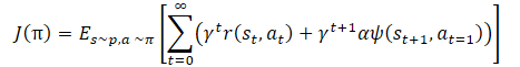
where γ is a discount factor,
      α — temperature ratio,
      ψ(St+1,At=1) — function of the subsequent state behavior (error of copying by the autoencoder).

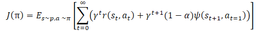
We again see the temperature ratio to regulate the balance between the model exploration and exploitation. This again leads to the above-described difficulties of hyperparameter tuning and model training. The method authors proposed to slightly change the policy training function.

The α temperature ratio itself should be determined using the following equation

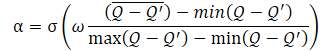
where σ is the sigmoid function,
      ω is equal to 10,
      Q — neural network for assessing the action quality.

The Q neural network used here is analogous to a critic and evaluates the quality of an action in a certain state taking into account the current policy.

As can be seen from the presented equation, the temperature ratio (1−α) ranges from 0 to 0.5. It increases as the assessment of the action quality improves. Obviously, at this moment, the error of data copying by the autoencoder tends to "0". With a high degree of probability, the model is currently in some kind of local minimum, and studying the environment can help get out of this state.

When the accuracy of data copying is low, the quality of the assessment of the action in a given state also decreases. This leads to an increase in the denominator of the expression inside the sigmoid function. Accordingly, the entire value of the sigmoid argument decreases, and its result tends to 0.5.

Keep in mind that we always subtract the smaller error from the larger one here. Therefore, the sigmoid argument is always greater than "0". It is almost never equal to "0", since we cannot divide by "0".

The presented algorithm is still a member of the large family of Actor-Critic algorithms and uses the general approaches of this family of algorithms. Like Soft Actor-Critic, the algorithm is used to learn Actor policies in a continuous action space. We will use 2 Critics models to evaluate the quality of the action and the distribution of the error gradient from reward to action. We will also use soft updating of target models, an experience buffer, and other general approaches to training Actor-Critic models.

2. Implementation using MQL5

After considering the theoretical aspects of the proposed approach, let's implement it using MQL5. The first thing we start with is the architecture of the models. To make the methods comparable, I did not change much the architecture of the models from the previous article. However, I simplified the Actor architecture a little and removed the complex last neural layer we created to implement the stochastic Actor algorithm from the Soft Actor-Critic method. However, I left the use of the stochastic Actor policy intact. But this time it is achieved by using the variational autoencoder latent state layer. As you remember, the input of this neural layer is supplied with a data tensor exactly two times the size of its results buffer. The specified source data tensor contains the mean and variance of the distribution for each element of the results. This way we reduce the computational complexity, but leave the stochastic Actor model in a continuous action space.

bool CreateDescriptions(CArrayObj *actor, CArrayObj *critic, CArrayObj *autoencoder)
  {
//---
   CLayerDescription *descr;
//---
   if(!actor)
     {
      actor = new CArrayObj();
      if(!actor)
         return false;
     }
   if(!critic)
     {
      critic = new CArrayObj();
      if(!critic)
         return false;
     }
   if(!autoencoder)
     {
      autoencoder = new CArrayObj();
      if(!autoencoder)
         return false;
     }
//--- Actor
   actor.Clear();
//--- Input layer
   if(!(descr = new CLayerDescription()))
      return false;
   descr.type = defNeuronBaseOCL;
   int prev_count = descr.count = (HistoryBars * BarDescr);
   descr.activation = None;
   descr.optimization = ADAM;
   if(!actor.Add(descr))
     {
      delete descr;
      return false;
     }
//--- layer 1
   if(!(descr = new CLayerDescription()))
      return false;
   descr.type = defNeuronBatchNormOCL;
   descr.count = prev_count;
   descr.batch = 1000;
   descr.activation = None;
   descr.optimization = ADAM;
   if(!actor.Add(descr))
     {
      delete descr;
      return false;
     }
//--- layer 2
   if(!(descr = new CLayerDescription()))
      return false;
   descr.type = defNeuronConvOCL;
   prev_count = descr.count = prev_count - 1;
   descr.window = 2;
   descr.step = 1;
   descr.window_out = 8;
   descr.activation = LReLU;
   descr.optimization = ADAM;
   if(!actor.Add(descr))
     {
      delete descr;
      return false;
     }
//--- layer 3
   if(!(descr = new CLayerDescription()))
      return false;
   descr.type = defNeuronConvOCL;
   prev_count = descr.count = prev_count;
   descr.window = 8;
   descr.step = 8;
   descr.window_out = 8;
   descr.activation = LReLU;
   descr.optimization = ADAM;
   if(!actor.Add(descr))
     {
      delete descr;
      return false;
     }
//--- layer 4
   if(!(descr = new CLayerDescription()))
      return false;
   descr.type = defNeuronBaseOCL;
   descr.count = 256;
   descr.optimization = ADAM;
   descr.activation = LReLU;
   if(!actor.Add(descr))
     {
      delete descr;
      return false;
     }
//--- layer 5
   if(!(descr = new CLayerDescription()))
      return false;
   descr.type = defNeuronBaseOCL;
   prev_count = descr.count = 128;
   descr.activation = LReLU;
   descr.optimization = ADAM;
   if(!actor.Add(descr))
     {
      delete descr;
      return false;
     }
//--- layer 6
   if(!(descr = new CLayerDescription()))
      return false;
   descr.type = defNeuronConcatenate;
   descr.count = LatentCount;
   descr.window = prev_count;
   descr.step = AccountDescr;
   descr.optimization = ADAM;
   descr.activation = SIGMOID;
   if(!actor.Add(descr))
     {
      delete descr;
      return false;
     }
//--- layer 7
   if(!(descr = new CLayerDescription()))
      return false;
   descr.type = defNeuronBaseOCL;
   descr.count = 256;
   descr.activation = LReLU;
   descr.optimization = ADAM;
   if(!actor.Add(descr))
     {
      delete descr;
      return false;
     }
//--- layer 8
   if(!(descr = new CLayerDescription()))
      return false;
   descr.type = defNeuronBaseOCL;
   descr.count = 256;
   descr.activation = LReLU;
   descr.optimization = ADAM;
   if(!actor.Add(descr))
     {
      delete descr;
      return false;
     }
//--- layer 9
   if(!(descr = new CLayerDescription()))
      return false;
   descr.type = defNeuronBaseOCL;
   descr.count = 2*NActions;
   descr.activation = LReLU;
   descr.optimization = ADAM;
   if(!actor.Add(descr))
     {
      delete descr;
      return false;
     }
//--- layer 10
   if(!(descr = new CLayerDescription()))
      return false;
   descr.type = defNeuronVAEOCL;
   descr.count = NActions;
   descr.optimization = ADAM;
   if(!actor.Add(descr))
     {
      delete descr;
      return false;
     }

The critic model has been transferred without changes, and we will not dwell on it.

Let's talk a little about the autoencoder model. As previously mentioned, the autoencoder is used as a memory element of the previously discussed "State-Action" pairs. We can call it the counter of the number of visits of these pairs. But let's remember that it is the "State-Action" pairs that our Critics evaluate. More precisely, the Critic evaluates an individual action in a specific state. This may seem a play on words and concepts, but one set of initial data.

Previously, to save resources and time for training models, we excluded the source data preprocessing block from the Critics architecture. Instead, we use already processed data from the hidden state of the Actor model. At the Critic’s input, we concatenate the hidden state and the Actor’s result buffer, thereby combining the state and action into one tensor.

Now we will go even further. We will feed the hidden state of one of the Critics as the input of our autoencoder. Similar to the Critic, we could use a concatenation layer of two tensors of the original data. But then we would have to solve the issue of comparing 1 buffer of autoencoder results with 2 buffers of source data. Using one buffer of source data from the Critic’s latent representation allows us to use a simpler autoencoder model and compare the source data with the results of its work "1:1". Thus, we will use only fully connected layers in the autoencoder architecture.

//--- Autoencoder
   autoencoder.Clear();
//--- Input layer
   if(!(descr = new CLayerDescription()))
      return false;
   descr.type = defNeuronBaseOCL;
   prev_count = descr.count = LatentCount;
   descr.activation = None;
   descr.optimization = ADAM;
   if(!autoencoder.Add(descr))
     {
      delete descr;
      return false;
     }
//--- layer 1
   if(!(descr = new CLayerDescription()))
      return false;
   descr.type = defNeuronBaseOCL;
   prev_count = descr.count = prev_count / 2;
   descr.optimization = ADAM;
   descr.activation = LReLU;
   if(!autoencoder.Add(descr))
     {
      delete descr;
      return false;
     }
//--- layer 2
   if(!(descr = new CLayerDescription()))
      return false;
   descr.type = defNeuronBaseOCL;
   prev_count = descr.count = prev_count / 2;
   descr.activation = LReLU;
   descr.optimization = ADAM;
   if(!autoencoder.Add(descr))
     {
      delete descr;
      return false;
     }
//--- layer 3
   if(!(descr = new CLayerDescription()))
      return false;
   descr.type = defNeuronBaseOCL;
   prev_count = descr.count = 20;
   descr.count = LatentCount;
   descr.activation = LReLU;
   descr.optimization = ADAM;
   if(!autoencoder.Add(descr))
     {
      delete descr;
      return false;
     }
//--- layer 4
   if(!(descr = new CLayerDescription()))
      return false;
   if(!(descr.Copy(autoencoder.At(2))))
     {
      delete descr;
      return false;
     }
   if(!autoencoder.Add(descr))
     {
      delete descr;
      return false;
     }
//--- layer 5
   if(!(descr = new CLayerDescription()))
      return false;
   if(!(descr.Copy(autoencoder.At(1))))
     {
      delete descr;
      return false;
     }
   if(!autoencoder.Add(descr))
     {
      delete descr;
      return false;
     }
//--- layer 6
   if(!(descr = new CLayerDescription()))
      return false;
   if(!(descr.Copy(autoencoder.At(0))))
     {
      delete descr;
      return false;
     }
   if(!autoencoder.Add(descr))
     {
      delete descr;
      return false;
     }
//---
   return true;
  }

Please note that starting from the fourth layer of the autoencoder, we did not completely create a description of the new neural layers. Instead, we simply copied the previously created descriptions in reverse order. This allowed us to create a mirror copy of the Encoder in the Decoder. Any changes in the Encoder architecture (except for adding new layers) will immediately be reflected in the corresponding Decoder layers. A rather convenient way to synchronize the description of neural layer architectures can be used in various cases.

After creating a description of the model architecture, we move on to arranging the process of collecting a database of examples for training the model. As before, this process is organized in the "..\BAC\Research.mq5" EA. The BAC method does not make any changes to the primary data collection algorithm. Therefore, the changes in this EA were minimal.

We have changed the function of describing the model architecture by adding a description of the Autoencoder to it. Consequently, when calling this function in the OnInit method of the Research.mq5 EA, we need to pass three pointers to dynamic arrays of descriptions of the model architecture. But since in this EA we will only use the Actor and we do not need a description of other models, we will not create an additional array of objects, but point out the array of descriptions of the Critic’s architecture two times. With such a call, a description of the Critic’s architecture will first be created in the function, then it will be deleted and the autoencoder architecture will be written to the array. In this case, this is not critical for us, since neither the critic nor the autoencoder model is used.

//+------------------------------------------------------------------+
//| Expert initialization function                                   |
//+------------------------------------------------------------------+
int OnInit()
  {
//---
........
........
//--- load models
   float temp;
   if(!Actor.Load(FileName + "Act.nnw", temp, temp, temp, dtStudied, true))
     {
      CArrayObj *actor = new CArrayObj();
      CArrayObj *critic = new CArrayObj();
      if(!CreateDescriptions(actor, critic, critic))
        {
         delete actor;
         delete critic;
         return INIT_FAILED;
        }
      if(!Actor.Create(actor))
        {
         delete actor;
         delete critic;
         return INIT_FAILED;
        }
      delete actor;
      delete critic;
      //---
     }
//---
........
........
//---
   return(INIT_SUCCEEDED);
  }

In addition, we exclude the entropy component from the reward function. The rest of the Expert Advisor code remained unchanged. You can find the full code of the EA and all its functions in the attachment.

The "..\BAC\Study.mq5" model training EA code required more work. Here we use and initialize all the models. Therefore, before calling the method for creating a description of the model architecture, we create an additional dynamic array for the Autoencoder.

int OnInit()
  {
//---
   ResetLastError();
   if(!LoadTotalBase())
     {
      PrintFormat("Error of load study data: %d", GetLastError());
      return INIT_FAILED;
     }
//--- load models
   float temp;
   if(!Actor.Load(FileName + "Act.nnw", temp, temp, temp, dtStudied, true) ||
      !Critic1.Load(FileName + "Crt1.nnw", temp, temp, temp, dtStudied, true) ||
      !Critic2.Load(FileName + "Crt2.nnw", temp, temp, temp, dtStudied, true) ||
      !Autoencoder.Load(FileName + "AEnc.nnw", temp, temp, temp, dtStudied, true) ||
      !TargetCritic1.Load(FileName + "Crt1.nnw", temp, temp, temp, dtStudied, true) ||
      !TargetCritic2.Load(FileName + "Crt2.nnw", temp, temp, temp, dtStudied, true))
     {
      CArrayObj *actor = new CArrayObj();
      CArrayObj *critic = new CArrayObj();
      CArrayObj *autoencoder = new CArrayObj();
      if(!CreateDescriptions(actor, critic, autoencoder))
        {
         delete actor;
         delete critic;
         delete autoencoder;
         return INIT_FAILED;
        }

After obtaining the model architecture, we initialize all models and control the operations.

      if(!Actor.Create(actor) || !Critic1.Create(critic) || !Critic2.Create(critic) ||
         !Autoencoder.Create(autoencoder))
        {
         delete actor;
         delete critic;
         delete autoencoder;
         return INIT_FAILED;
        }

Do not forget about the critics' target models.

      if(!TargetCritic1.Create(critic) || !TargetCritic2.Create(critic))
        {
         delete actor;
         delete critic;
         delete autoencoder;
         return INIT_FAILED;
        }
      delete actor;
      delete critic;
      delete autoencoder;
      //---
      TargetCritic1.WeightsUpdate(GetPointer(Critic1), 1.0f);
      TargetCritic2.WeightsUpdate(GetPointer(Critic2), 1.0f);
     }

After that, make sure to transfer all models into one OpenCL context. Autoencoder is no exception.

   OpenCL = Actor.GetOpenCL();
   Critic1.SetOpenCL(OpenCL);
   Critic2.SetOpenCL(OpenCL);
   TargetCritic1.SetOpenCL(OpenCL);
   TargetCritic2.SetOpenCL(OpenCL);
   Autoencoder.SetOpenCL(OpenCL);

Next comes the model correspondence check block.

   Actor.getResults(Result);
   if(Result.Total() != NActions)
     {
      PrintFormat("The scope of the actor does not match the actions count (%d <> %d)", NActions, Result.Total());
      return INIT_FAILED;
     }
//---
   Actor.GetLayerOutput(0, Result);
   if(Result.Total() != (HistoryBars * BarDescr))
     {
      PrintFormat("Input size of Actor doesn't match state description (%d <> %d)", Result.Total(), 
                                                                                        (HistoryBars * BarDescr));
      return INIT_FAILED;
     }
//---
   Actor.GetLayerOutput(LatentLayer, Result);
   int latent_state = Result.Total();
   Critic1.GetLayerOutput(0, Result);
   if(Result.Total() != latent_state)
     {
      PrintFormat("Input size of Critic doesn't match latent state Actor (%d <> %d)", Result.Total(), latent_state);
      return INIT_FAILED;
     }

Here we add a check for consistency between the Autoencoder and Critic architectures.

   Critic1.GetLayerOutput(1, Result);
   latent_state = Result.Total();
   Autoencoder.GetLayerOutput(0, Result);
   if(Result.Total() != latent_state)
     {
      PrintFormat("Input size of Autoencoder doesn't match latent state Critic (%d <> %d)", Result.Total(), latent_state);
      return INIT_FAILED;
     }

At the end of the method, we, as before, initialize the auxiliary buffer and call the model training event.

   Gradient.BufferInit(AccountDescr, 0);
//---
   if(!EventChartCustom(ChartID(), 1, 0, 0, "Init"))
     {
      PrintFormat("Error of create study event: %d", GetLastError());
      return INIT_FAILED;
     }
//---
   return(INIT_SUCCEEDED);
  }

You might notice that we have not created an additional model for assessing the quality of action for the function of dynamic calculation of the temperature ratio. I have emphasized that the functionality of this model is similar to the work of the Critic. To simplify the overall training process, we will use the models of our critics in implementing the dynamic calculation of the temperature ratio.

After creating the models, do not forget to save the trained models in the EA's OnDeinit deinitialization method. Here we pay attention to the preservation of all models, as well as to the suffixes of file names and the corresponding models specified during the download.

void OnDeinit(const int reason)
  {
//---
   TargetCritic1.WeightsUpdate(GetPointer(Critic1), Tau);
   TargetCritic2.WeightsUpdate(GetPointer(Critic2), Tau);
   Actor.Save(FileName + "Act.nnw", 0, 0, 0, TimeCurrent(), true);
   TargetCritic1.Save(FileName + "Crt1.nnw", Critic1.getRecentAverageError(), 0, 0, TimeCurrent(), true);
   TargetCritic1.Save(FileName + "Crt2.nnw", Critic2.getRecentAverageError(), 0, 0, TimeCurrent(), true);
   Autoencoder.Save(FileName + "AEnc.nnw", Autoencoder.getRecentAverageError(), 0, 0, TimeCurrent(), true);
   delete Result;
  }

At this point, the preparatory work is completed, and we can move on to implementing the direct model training algorithm in the Train method of our EA.

The beginning of the method is pretty standard. As before, we arrange a training cycle with the number of iterations specified in the EA external parameters.

void Train(void)
  {
   int total_tr = ArraySize(Buffer);
   uint ticks = GetTickCount();
//---
   for(int iter = 0; (iter < Iterations && !IsStopped()); iter ++)
     {
      int tr = (int)((MathRand() / 32767.0) * (total_tr - 1));
      int i = (int)((MathRand() * MathRand() / MathPow(32767, 2)) * (Buffer[tr].Total - 2));

In the body of the loop, we randomly determine a trajectory from the example database and a specific trajectory step. Then we load information about the subsequent state into the data buffers.

      //--- Target
      State.AssignArray(Buffer[tr].States[i + 1].state);
      float PrevBalance = Buffer[tr].States[i].account[0];
      float PrevEquity = Buffer[tr].States[i].account[1];
      Account.Clear();
      Account.Add((Buffer[tr].States[i + 1].account[0] - PrevBalance) / PrevBalance);
      Account.Add(Buffer[tr].States[i + 1].account[1] / PrevBalance);
      Account.Add((Buffer[tr].States[i + 1].account[1] - PrevEquity) / PrevEquity);
      Account.Add(Buffer[tr].States[i + 1].account[2]);
      Account.Add(Buffer[tr].States[i + 1].account[3]);
      Account.Add(Buffer[tr].States[i + 1].account[4] / PrevBalance);
      Account.Add(Buffer[tr].States[i + 1].account[5] / PrevBalance);
      Account.Add(Buffer[tr].States[i + 1].account[6] / PrevBalance);
      double x = (double)Buffer[tr].States[i + 1].account[7] / (double)(D'2024.01.01' - D'2023.01.01');
      Account.Add((float)MathSin(x != 0 ? 2.0 * M_PI * x : 0));
      x = (double)Buffer[tr].States[i + 1].account[7] / (double)PeriodSeconds(PERIOD_MN1);
      Account.Add((float)MathCos(x != 0 ? 2.0 * M_PI * x : 0));
      x = (double)Buffer[tr].States[i + 1].account[7] / (double)PeriodSeconds(PERIOD_W1);
      Account.Add((float)MathSin(x != 0 ? 2.0 * M_PI * x : 0));
      x = (double)Buffer[tr].States[i + 1].account[7] / (double)PeriodSeconds(PERIOD_D1);
      Account.Add((float)MathSin(x != 0 ? 2.0 * M_PI * x : 0));
      //---
      if(Account.GetIndex() >= 0)
         Account.BufferWrite();

Next, we perform a forward pass of the Actor and 2 target Critics models to determine the value of the future state taking into account the updated Actor strategy.

      if(!Actor.feedForward(GetPointer(State), 1, false, GetPointer(Account)))
        {
         PrintFormat("%s -> %d", __FUNCTION__, __LINE__);
         ExpertRemove();
         break;
        }
      //---
      if(!TargetCritic1.feedForward(GetPointer(Actor), LatentLayer, GetPointer(Actor)) ||
         !TargetCritic2.feedForward(GetPointer(Actor), LatentLayer, GetPointer(Actor)))
        {
         PrintFormat("%s -> %d", __FUNCTION__, __LINE__);
         break;
        }
      TargetCritic1.getResults(Result);
      float reward = Result[0];
      TargetCritic2.getResults(Result);
      reward = Buffer[tr].Revards[i] + DiscFactor * (MathMin(reward, Result[0]) - Buffer[tr].Revards[i + 1]);

At first glance, everything is the same as when using the Soft Actor-Critic algorithm. We also use the minimum condition assessment received from two Critics. But note that we have excluded the entropy component. This is quite logical in light of the use of the BAC method. However, we have not added a behavioral component. This is a deliberate departure from the original algorithm. The fact is that we use a database of examples obtained as a result of passes of Actors with various policies. Introducing a behavioral component now will distort the Critic’s assessment, but will not directly stimulate the Actor. Later, we will receive indirect stimulation of the Actor when it is trained based on the assessments of Critics. But there is another side of the coin. What is the correspondence between the number of times the "State-Action" pair is used when training a Critic and the same or similar "State-Action" pair when training an Actor? A bias is possible in favor of one or another direction. Therefore, I decided to use the Autoencoder to estimate states and actions when training the Actor. In my opinion, this will make it possible to more accurately assess the frequency of visits to states and the actions used by the Actor, taking into account the update of its behavior policy.

The next stage is training the Critics. Load the data of the selected state from the example database into the data buffers.

      //--- Q-function study
      State.AssignArray(Buffer[tr].States[i].state);
      PrevBalance = Buffer[tr].States[MathMax(i - 1, 0)].account[0];
      PrevEquity = Buffer[tr].States[MathMax(i - 1, 0)].account[1];
      Account.Update(0, (Buffer[tr].States[i].account[0] - PrevBalance) / PrevBalance);
      Account.Update(1, Buffer[tr].States[i].account[1] / PrevBalance);
      Account.Update(2, (Buffer[tr].States[i].account[1] - PrevEquity) / PrevEquity);
      Account.Update(3, Buffer[tr].States[i].account[2]);
      Account.Update(4, Buffer[tr].States[i].account[3]);
      Account.Update(5, Buffer[tr].States[i].account[4] / PrevBalance);
      Account.Update(6, Buffer[tr].States[i].account[5] / PrevBalance);
      Account.Update(7, Buffer[tr].States[i].account[6] / PrevBalance);
      x = (double)Buffer[tr].States[i].account[7] / (double)(D'2024.01.01' - D'2023.01.01');
      Account.Add((float)MathSin(x != 0 ? 2.0 * M_PI * x : 0));
      x = (double)Buffer[tr].States[i].account[7] / (double)PeriodSeconds(PERIOD_MN1);
      Account.Add((float)MathCos(x != 0 ? 2.0 * M_PI * x : 0));
      x = (double)Buffer[tr].States[i].account[7] / (double)PeriodSeconds(PERIOD_W1);
      Account.Add((float)MathSin(x != 0 ? 2.0 * M_PI * x : 0));
      x = (double)Buffer[tr].States[i].account[7] / (double)PeriodSeconds(PERIOD_D1);
      Account.Add((float)MathSin(x != 0 ? 2.0 * M_PI * x : 0));
      Account.BufferWrite();

Now it is time to carry out the direct passage of the Actor. Let me remind you that in this case we use it for preliminary processing of initial data on the environment state.

      if(!Actor.feedForward(GetPointer(State), 1, false, GetPointer(Account)))
        {
         PrintFormat("%s -> %d", __FUNCTION__, __LINE__);
         break;
        }

Then we need to perform a forward and backward pass of the Critics to adjust their parameters. When training models using the Soft Actor-Critic method, we used model alternation. In this case, we will simultaneously train both Critics using the same examples. We call Critics' direct pass methods for actions from the example database.

      Actions.AssignArray(Buffer[tr].States[i].action);
      if(Actions.GetIndex() >= 0)
         Actions.BufferWrite();
      //---
      if(!Critic1.feedForward(GetPointer(Actor), LatentLayer, GetPointer(Actions)) ||
         !Critic2.feedForward(GetPointer(Actor), LatentLayer, GetPointer(Actions)))
        {
         PrintFormat("%s -> %d", __FUNCTION__, __LINE__);
         break;
        }

But before we do the reverse pass, we will prepare the data to calculate the temperature ratio of the behavioral component of our reward function. First, we compare the first Critic's estimation results with the future state estimate calculated above and update the minimum, maximum and average error values.

Note that we simply transfer the current error to all three variables for the first iteration. Then we update the maximum and minimum based on the comparison results. Then we calculate the exponential average.

      Critic1.getResults(Result);
      float error = reward - Result[0];
      if(iter == 0)
        {
         MaxCriticError = error;
         MinCriticError = error;
         AvgCriticError = error;
        }
      else
        {
         MaxCriticError = MathMax(error, MaxCriticError);
         MinCriticError = MathMin(error, MinCriticError);
         AvgCriticError = 0.99f * AvgCriticError + 0.01f * error;
        }

For the second Critic, we already have the initial values of the variables. We update their values regardless of the model training iteration.

      Critic2.getResults(Result);
      error = reward - Result[0];
      MaxCriticError = MathMax(error, MaxCriticError);
      MinCriticError = MathMin(error, MinCriticError);
      AvgCriticError = 0.99f * AvgCriticError + 0.01f * error;

At the end of updating the parameters of the Critics, all we have to do is perform a backward pass of both models, indicating the minimum estimate of the future state from the target models as a reference value.

      Result.Update(0, reward);
      if(!Critic1.backProp(Result, GetPointer(Actions), GetPointer(Gradient)) ||
         !Critic2.backProp(Result, GetPointer(Actions), GetPointer(Gradient)))
        {
         PrintFormat("%s -> %d", __FUNCTION__, __LINE__);
         break;
        }

This completes the update of the critics' parameters, and we move on to training the Actor. The authors of the BAC method for training the Actor recommend using the Critic with a minimum assessment of the selected action. To avoid carrying out a direct pass through two Critics and comparing their results, we will do things a little differently. We will take a Critic with the minimum average error in predicting the state and action assessment. This value is re-estimated with each return pass of the Critic's model. Its extraction will require minimal costs, which are negligible compared to carrying out a direct pass through the model.

To avoid creating complex branched structures with repetition of actions for one and the second Critic model, we will simply save the pointer to the desired model in a local variable. Then we will work with this local variable.

      //--- Policy study
      CNet *critic = NULL;
      if(Critic1.getRecentAverageError() <= Critic2.getRecentAverageError())
         critic = GetPointer(Critic1);
      else
         critic = GetPointer(Critic2);

Unlike TD3, Actor-Critic methods update the Actor policy at each iteration. We will use the same set of initial data that we chose to train the Critics. Let me remind you that while training Critics, we have already carried out a direct pass of the Actor with the current set of initial data. Therefore, it is sufficient to carry out a direct pass of the selected Critic to evaluate the actions of the Actor in the current state, taking into account the update of its policy.

      if(!critic.feedForward(GetPointer(Actor), LatentLayer, GetPointer(Actor)) ||
         !Autoencoder.feedForward(critic, 1, NULL, -1))
        {
         PrintFormat("%s -> %d", __FUNCTION__, __LINE__);
         break;
        }

After the forward pass of the Critic, we perform a forward pass of the Autoencoder. Here is a nuance. The fact is that earlier, linking the two models into a single whole, we added the replacement of the source data layer of the subsequent model with the pointer to the latent layer of the model that provides these source data. This works great when we use one Actor as a donor for two Critics. During the first iteration, Critics remove the unnecessary source data layer and store a pointer to the Actor's latent state layer. In the case of Autoencoder, we have the opposite situation. We use 2 Critic models as donors for one Autoencoder. At the first iteration, the Autoencoder removes the unnecessary layer of the original data and stores a pointer to the latent layer of the used Critic. But when changing the Critic, the layer of one Critic will be deleted and the pointer to the layer of another Critic will be saved. This process is extremely undesirable for us. Moreover, it is detrimental to our entire training. Therefore, after the first deletion of the source data layer, we need to disable the object deletion flag when updating the neural layer array.

bool CNet::feedForward(CNet *inputNet, int inputLayer = -1, CNet *secondNet = NULL, int secondLayer = -1)
  {
........
........
//---
   if(layer.At(0) != neuron)
      if(!layer.Update(0, neuron))
        {
         if(del_second)
            delete second;
         return false;
        }
      else
         layer.FreeMode(false);
//---
........
........
//---
   return true;
  }

This is a small departure from the training process and the BAC algorithm, but it is critical to our implementation of the process design.

Let's return to the algorithm of our Train model training method. After a direct pass of the Autoencoder, we have to evaluate the error of data copying. To do this, we load the result of the Autoencoder and the initial data from the latent state of the Critic. To increase the efficiency of our code, we will use vector variables both data buffers will be loaded into.

      Autoencoder.getResults(AutoencoderResult);
      critic.GetLayerOutput(1, Result);
      Result.GetData(CriticResult);

Here we will immediately upload the results of the Critic’s assessment of actions.

      critic.getResults(Result);

We need both streams of information to determine the target value when training the Actor policy. Therefore, we will combine the entire calculation in one block.

Previously, we prepared data for calculating the temperature ratio. Now we will first calculate the sigmoid argument. Then we determine the value of the function and subtract it from "1".

      float alpha = (MaxCriticError == MinCriticError ? 0 : 
                                       10.0f * (AvgCriticError - MinCriticError) / (MaxCriticError - MinCriticError));
      alpha = 1.0f / (1.0f + MathExp(-alpha));
      alpha = 1 - alpha;
      reward = Result[0];
      reward = (reward > 0 ? reward + PoliticAdjust : PoliticAdjust);
      reward += AutoencoderResult.Loss(CriticResult, LOSS_MSE) * alpha;

Next, similar to the approaches in TD3, we shift the Actor parameters towards increasing the profitability of operations. Therefore, we add a small constant to the current assessment of the action, stimulating a shift in gradients towards increasing profitability.

To complete the formation of the target value, we add the behavioral component taking into account the loss function of the Autoencoder. Thanks to vector operations, the size of the loss function, is literally defined in a single string regardless of the size of the data buffers.

Now, after generating the target value, we can perform a reverse pass of the Critic and the Actor to distribute the error gradient before the action and subsequent adjustment of the Actor’s parameters.

As before, to prevent mutual adjustment of the parameters of the Critic and Actor, before performing the reverse pass, we turn off the Critic’s training mode and turn it back on after performing the operations.

      Result.Update(0, reward);
      critic.TrainMode(false);
      if(!critic.backProp(Result, GetPointer(Actor)) ||
         !Actor.backPropGradient(GetPointer(Account), GetPointer(Gradient), LatentLayer) ||
         !Actor.backPropGradient(GetPointer(Account), GetPointer(Gradient)))
        {
         PrintFormat("%s -> %d", __FUNCTION__, __LINE__);
         critic.TrainMode(true);
         break;
        }
      critic.TrainMode(true);

Note that we are doing two types of backpass for the Actor. We first distribute the error gradient across the data preprocessing unit, which will allow us to fine-tune the filters of the convolutional layers based on the Critics' requirements. Then we carry out a reverse pass to adjust the decision-making block on choosing a specific action. It is very important to carry out operations in this sequence. After a complete forward pass with adjustment of the parameters of the decision-making block, the error gradients for the data preliminary processing block will also be rewritten. In this case, calling an additional return pass will not have a positive effect. Moreover, it may also have a negative effect.

At this stage, we have updated the Critics and Actor parameters. All we have to do is update the Autoencoder parameters. Everything is quite simple here. We pass the Critic's latent state data as reference values and perform a backward pass through the model.

      //--- Autoencoder study
      Result.AssignArray(CriticResult);
      if(!Autoencoder.backProp(Result, critic, 1))
        {
         PrintFormat("%s -> %d", __FUNCTION__, __LINE__);
         break;
        }

At the end of the training cycle iterations, we update the target models of both Critics and inform the user about the progress of the training.

      //--- Update Target Nets
      TargetCritic1.WeightsUpdate(GetPointer(Critic1), Tau);
      TargetCritic2.WeightsUpdate(GetPointer(Critic2), Tau);
      //---
      if(GetTickCount() - ticks > 500)
        {
         string str = StringFormat("%-15s %5.2f%% -> Error %15.8f\n", "Critic1", 
                                   iter * 100.0 / (double)(Iterations), Critic1.getRecentAverageError());
         str += StringFormat("%-15s %5.2f%% -> Error %15.8f\n", "Critic2", 
                                   iter * 100.0 / (double)(Iterations), Critic2.getRecentAverageError());
         Comment(str);
         ticks = GetTickCount();
        }
     }

The ending of the training method is pretty conventional:

• clear the comment field,
• display training results,
• initialize the end of the EA's work.

   Comment("");
//---
   PrintFormat("%s -> %d -> %-15s %10.7f", __FUNCTION__, __LINE__, "Critic1", Critic1.getRecentAverageError());
   PrintFormat("%s -> %d -> %-15s %10.7f", __FUNCTION__, __LINE__, "Critic2", Critic2.getRecentAverageError());
   ExpertRemove();
//---
  }

The complete code of the training EA and all programs used can be found in the attachment. There you will also find the code for the testing EA, which was carried over from the previous article almost unchanged. Only the entropy component has been removed in the EA code while maintaining the traversed trajectory.

With this, we complete the work on building EAs and move on to testing the work done and training models.

In my opinion, the work resulted in a fairly large number of iterations of data exchange between the main memory and the OpenCL context. This is noticeable in the block for determining the behavioral component of the reward function. There is something to think about here. Let's see how this affects the overall performance of the model training.

3. Test

We have done quite an impressive work on implementing the Behavior-Guided Actor-Critic algorithm, and now it is time to look at the results. As before, the models were trained on EURUSD H1 on the first 5 months of 2023. All indicator parameters are used by default. The initial balance is USD 10,000.

At the first stage, a training set of 300 random passes was created, which gave more than 750 thousand separate sets of "State → Action → New state → Reward" data. Mind that I have mentioned the "random passes" here. We do not have a pre-trained model at this stage. With each pass in the strategy tester, the "..\BAC\Research.mq5" EA generates a new model and fills it with random parameters. Accordingly, the operation of such models will be as random as their parameters. At this stage, I did not limit the level of minimum profitability of a pass to save examples to the database.

After collecting examples, we carry out initial training of our model. To do this, we run the "..\BAC\Study.mq5" EA for 500,000 iterations of model training.

I must say that after the initial training of the model, the stochasticity of the Actor’s policy is felt quite strongly. This is reflected in the wide spread of results of individual passes.

At the second stage, we re-launch the training data collection EA in the optimization mode of the strategy tester for 300 iterations with a complete search of parameters. This time we limit the minimum return level to positive results (0 or slightly higher). As a result, a relatively small number of results were added (15-20 passes).

Please note that when running the Data Collection EA after initial training, all passes use the same pre-trained model. The entire spread of results is due to the stochasticity of the Actor’s policy.

Next, we re-run the model training process for the same 500,000 iterations.

Collecting examples and training the model are repeated several times until the desired result is obtained or a local minimum is reached when the next iteration of collecting examples and training the model does not produce any progress.

Note that the previously collected passes are not deleted during the next run of the example database collection EA. The new ones are added to the end of the file. The MaxReplayBuffer constant was added to the "..\BAC\Trajectory.mqh" file to prevent the accumulation of too large database of examples. This constant specifies the maximum number of passes (not the file size). As the buffer fills, older passes will be deleted. I recommend that you use this constant to adjust the size of the example database in accordance with the technical capabilities of your equipment.

#define                    MaxReplayBuffer 500

After about 7 iterations of updating the example database and training the model, I was able to get a model capable of generating profit on the training time interval. The presented graph clearly shows a tendency towards capital growth. However, there are also some unprofitable areas.

Over the 5 months of the training period, the EA earned 16% profit with a maximum drawdown of 8.41% in Equity. On the balance sheet, the drawdown was slightly lower and amounted to 6.68%. In total, 99 trades were made, 51.5% of them were closed with a profit. The number of profitable trades is almost equal to the number of unprofitable ones. But the average winning trade is almost 50% larger than the average losing trade. The profit factor was 1.53 and the recovery factor indicator was almost at the same level.

However, we train the model to be used in the future, and not just in the strategy tester. Therefore, testing the model on data outside the training set is more important for us. We tested the same model on historical data of June 2023. All other testing parameters remained unchanged.

The results of testing the model on new data are comparable to the results on the training set. In 1 month, the EA earned a little more than 3% profit, which is quite comparable to 16% in 5 months of the training sample. 11 trades were made, which is lower than the corresponding indicator on the training sample. Unfortunately, the share of profitable trades is also lower than the training sample and amounted to only 36.4%. However, the average profitable trade is almost 6 times higher than the average losing one. Thanks to this, the profit factor increased to 3.12.

Conclusion

In this article, we considered another algorithm for training Behavior-Guided Actor-Critic models. Like the Soft Actor-Critic method, it belongs to the large family of Actor-Critic algorithms and is an alternative to using the Soft Actor-Critic method. The advantages of the considered algorithm include the ability to train both stochastic and deterministic models in a continuous action space. The use of this method does not carry any restrictions in the construction of trained models.

In the practical part of this article, the proposed algorithm was implemented using MQL5. The efficiency of our implementation is confirmed by testing results.

Let me say once again that all the programs presented only demonstrate the possibility of using the technology. They are not ready for use in real financial markets. The EAs need to be refined and additionally tested before being launched on a real market.

Links

Behavior-Guided Actor-Critic: Improving Exploration via Learning Policy Behavior Representation for Deep Reinforcement Learning

Neural networks made easy (Part 49): Soft Actor-Critic

Neural networks made easy (Part 50): Soft Actor-Critic (model optimization)

Programs used in the article

#	Name	Type	Description
1	Research.mq5	Expert Advisor	Example collection EA
2	Study.mq5	Expert Advisor	Agent training EA
3	Test.mq5	Expert Advisor	Model testing EA
4	Trajectory.mqh	Class library	System state description structure
5	NeuroNet.mqh	Class library	A library of classes for creating a neural network
6	NeuroNet.cl	Code Base	OpenCL program code library