Neural networks made easy (Part 33): Quantile regression in distributed Q-learning

MetaTrader 5 — Trading systems | 17 March 2023, 14:31

4 226

Dmitriy Gizlyk

Introduction

In the previous article, we got acquainted with distributed Q-learning, which allows learning the probability distribution of the predicted reward. We have learned how to predict the probability of receiving the expected reward in a specific value range. But the number of such ranges and the spread of reward values are hyperparameters of the model. Therefore, expert knowledge about the distribution of reward values is required in order to select the optimal parameters. We also need to conduct certain tests to select optimal hyperparameters.

It must say that the approach to divide the entire range of possible values into equal ranges, which we considered previous time, also has its drawbacks. We identified one neuron to predict the probability of receiving a reward in each of the individual ranges for each action. However, in practice, quite often the probability of receiving a reward in a large number of ranges is equal to 0. This means that we are using our resources inefficiently. We could combine some ranges to reduce the number of operations. This would speed up the model training and execution. At the same time, the probability of receiving rewards in other ranges is quite high. To get a more complete picture, we could break this range into smaller components. This would improve the accuracy of predicting the expected reward. However, our approach does not allow the creation of different size ranges. These drawbacks can be solved by using the quantile regression algorithm proposed in October 2017 in the article "Distributional Reinforcement Learning with Quantile Regression".

1. Quantile Regression

Quantile regression models the relationship between the distribution of the explanatory variables and certain quantiles of the target variable.

Before we proceed to considering the use of quantile regression in distributed Q-learning, it should be mentioned that the proposed algorithm approaches the evaluation of the probabilistic distribution of the expected reward from the other side. Previously, we divided the range of possible reward values into different sections. In the new algorithm, we divide the set of rewards received into several equally probable quantiles. What are the benefits of this?

We still have a hyperparameter for the number of analyzed quantiles. But at the same time, we do not limit the range of possible reward values. Instead, we train our model to predict the median values of the quantiles. Since we are using equiprobable quantiles, we will not have quantiles with zero-probability rewards. Moreover, in the area of sparse reward values, we will get larger quantiles. In areas where there will be lots of rewards, quantiles will be broken down into smaller parts. Thereby, we get a more complete picture of the probability distribution of the expected reward. Moreover, this approach enables the identification of non-static areas of sparse and increased density of reward values. They may vary depending on the state of the environment.

However, it remains the same Q-learning. The process itself is based on the Bellman optimization equation.

Bellman optimization equation

However, this time we have to define not one value, but the whole distribution. But basically, the task remains the same. Let's take a closer look at the task.

As mentioned above, we split the entire reward distribution of the training sample into N equiprobable quantiles. Each quantile is the level which is not exceeded by the analyzed random variable with a given probability. Here equally probable quantiles are the quantiles with a fixed step, while the total set of them covers the entire training dataset.

In practice, when we have a training dataset, the probability of getting one of the elements from the dataset 1. There cannot be any other option because all elements are taken from the training dataset.

Splitting the set into N equiprobable quantiles implies splitting the entire training dataset into N equal parts. Each of them will contain the same number of elements. The probability of choosing an element from one of the subsets is 1/N.

A separate quantile is characterized by 2 parameters: the probability of selecting an element and the upper limit of its element values. An additional condition for quantiles is their sorting in ascending order with the accumulation of probabilities. It means that the upper limit of the values of each subsequent quantile is higher than the previous one. The probability of a quantile includes the probability of previous quantiles. For example, for a certain distribution, we have a quantile of 0.2 with a level of 15. This means that the value of 20% of the elements of the entire distribution does not exceed 15. The step of probabilities and the level of the maximum quantile values may not be proportional as they depend on the specific distribution.

The algorithm we are considering involves splitting the dataset into quantiles with a fixed probability step. Instead of upper limits, we will train the model to predict the median values of the quantiles.

To train the model, we need target values. Having a complete set of elements of a certain dataset, we can easily find the average value.

But we do not have a complete set in practice. We receive rewards from the environment only after performing an action and transiting to a new state. As you can see, the use of a new model training algorithm does not affect the interaction with the environment. In the original Q-learning, we trained the model to predict the average expected reward. We did this by iteratively shifting the results of our model to the target values with a small learning coefficient. As you can see, during the learning process, our model result is constantly affected by a shift force towards the current target value. The average value is reached at the moment when the multidirectional forces balance each other (as shown in the figure).

We can use a similar approach in solving problems of the new algorithm. But there is one thing. This algorithm allows you to can find the average value of the set. This is a quantile of 0.5. When applying it in its purest form, we will get the same values on all neurons of the model's results layer. They will all work synchronously, like one neuron. However, we need to obtain the true distribution of values over the analyzed quantiles.

Look at the nature of the quantile. For example, consider a quantile of 0.25, which is a quarter of the analyzed dataset. If we discard the distance between the values of the elements, then for every 1 element of the quantile there should be 3 elements from the total set that do not fall into this quantile. Returning to our example above, in order to achieve equilibrium at the 0.25 quantile point, the force of value decrease must be 3 times the force of the value increase for the quantile.

Therefore, to find the value of each specific quantile, we should just introduce a correction factor into the Bellman equation. The factor will depend on the quantile level and the direction of the deviation.

where τ is the probabilistic characteristic of the quantile.

In the learning process, we use all the heuristics of the classical Q-learning algorithm in the form of experience reproduction and Target Net.

2. Implementation in MQL5

After considering the theoretical aspects of the algorithm, let us move on to the practical part of our article. We will consider how to implement the algorithm using MQL5. While implementing the algorithm, we will not create new architectures of neural layers. However, we will move the process organization into a separate class, CQRDQN. This will simplify the use of the method in Expert Advisors and will protect the user from some implementation details. The structure of the new class is shown below.

class CQRDQN : protected CNet
  {
private:
   uint              iCountBackProp;
protected:
   uint              iNumbers;
   uint              iActions;
   uint              iUpdateTarget;
   matrix<float>     mTaus;
   //---
   CNet              cTargetNet;
public:
   /** Constructor */
                     CQRDQN(void);
                     CQRDQN(CArrayObj *Description)  { Create(Description, iActions); }
   bool              Create(CArrayObj *Description, uint actions);
   /** Destructor */~CQRDQN(void);
   bool              feedForward(CArrayFloat *inputVals, int window = 1, bool tem = true) 
                       { return        CNet::feedForward(inputVals, window, tem); }
   bool              backProp(CBufferFloat *targetVals, float discount,
                              CArrayFloat *nextState, int window = 1, bool tem = true); 
   void              getResults(CBufferFloat *&resultVals);
   int               getAction(void); 
   int               getSample(void);
   float             getRecentAverageError() { return recentAverageError; } 
   bool              Save(string file_name, datetime time, bool common = true)
                       { return        CNet::Save(file_name, getRecentAverageError(),
                                                  (float)iActions, 0, time, common); }
   virtual bool      Save(const int file_handle);
   virtual bool      Load(string file_name, datetime &time, bool common = true);
   virtual bool      Load(const int file_handle);
   //---
   virtual int       Type(void)   const   {  return defQRDQN;   }
   virtual bool      TrainMode(bool flag) { return CNet::TrainMode(flag); } 
   virtual bool      GetLayerOutput(uint layer, CBufferFloat *&result) 
     { return        CNet::GetLayerOutput(layer, result); }
   //---
   virtual void      SetUpdateTarget(uint batch)   { iUpdateTarget = batch; }
   virtual bool      UpdateTarget(string file_name);
   //---
   virtual bool      SetActions(uint actions);
  };

The new class is derived from the CNet class that organizes the work of our neural network models. This means that we will build a new algorithm for operating with the model.

To store the key parameters of our algorithm, we will create the following variables:

iNumbers — the number of neurons in the set describing the distribution of one action
iActions — the number of possible action variants
iUpdateTarget — frequency of updating model parameters Target Net
mTaus — matrix for writing probabilistic characteristics of quantiles
cTargetNet — pointer to the Target Net object

Pay attention that in the mTaus matrix we write down the median values of the probabilities of each quantile.

In the class constructor, set the initial values for these variables.

CQRDQN::CQRDQN()  :  iNumbers(31),
                     iActions(2),
                     iUpdateTarget(1000)
  {
   mTaus = matrix<float>::Ones(1, iNumbers) / iNumbers;
   mTaus[0, 0] /= 2;
   mTaus = mTaus.CumSum(0);
   cTargetNet.Create(NULL);
   Create(NULL, iActions);
  }

As in the CNet class that organizes the neural network model, in addition to the constructor without parameters, we will create a method overload with the specification of the architecture of the model we are creating.

                     CQRDQN(CArrayObj *Description)  { Create(Description, iActions); }

The method will be created in the Create method. The method receives in parameters a pointer to an array that describing the model architecture and the number of the agent's possible actions.

bool CQRDQN::Create(CArrayObj *Description, uint actions)
  {
   if(actions <= 0 || !CNet::Create(Description))
      return false;

In the method body, check whether the number of agent actions is specified correctly. Call the parent class method which has the same name. It includes all the necessary controls regarding the object describing the model architecture as well as implements the model creation process. Here we only check the logical result of the parent class operations.

After successfully creating a new model, take the results layer of the created model. Based on information about its size and the number of possible agent actions, fill in the mTaus matrix of probabilistic quantile characteristics. The number of rows in this matrix is equal to the size of the probability distribution of the reward for one action. Since the probabilities of each quantile, which are set before the start of training, are equal for all possible actions of the agent with an equal fixed step, we will use a vector matrix with one row. We use a matrix rather than a vector because the solution will be developed further, and later it may imply variable probability distributions for actions.

   int last_layer = Description.Total() - 1;
   CLayer *layer = layers.At(last_layer);
   if(!layer)
      return false;
   CNeuronBaseOCL *neuron = layer.At(0);
   if(!neuron)
      return false;
   iActions = actions;
   iNumbers = neuron.Neurons() / actions;
   mTaus = matrix<float>::Ones(1, iNumbers) / iNumbers;
   mTaus[0, 0] /= 2;
   mTaus = mTaus.CumSum(0);
   cTargetNet.Create(NULL);
//---
   return true;
  }

Note that at the initial step we reset Target Net. This approach prevents the training of a new model on absolutely random values of an untrained model.

To implement the feed forward pass, we will use a similar method of the parent class.

   bool              feedForward(CArrayFloat *inputVals, int window = 1, bool tem = true) 
                     { return CNet::feedForward(inputVals, window, tem); }

As for the feed backward method backProp, we need to work with it a little. Let me remind you that the environment reacts to each agent action with a reward. In the classical Q-learning process, we have defined a reward policy. Since possible agent actions in trading are mutually exclusive and are opposite in nature, we can determine the reward for the opposite action by the reward which the environment returned for the action performed. Based on this feature, we can pass the target values for all possible actions at each iteration of the feed backward pass. This makes the learning process faster and more stable. But in the distributed Q-learning process we are dealing with a whole vector of target values for each action. In the previous article, we built a new process for creating a model target tensor in the model training EA. We also created a new block for decoding the model results before performing an action in the trading EA to check how the trained model works.

Now, by creating a new class, we can hide this process from the user. Thus, working with the model will be simpler and clearer. Actually, it will be similar to working with the classical Q-learning, in which the environment returns only a discrete reward value per action, while the whole process of converting this discrete reward into a distribution vector for each action is implemented in the body of the feed backward method.

I must say about one more advantage of using a new class to implement the process. As you know, Q-learning process uses Target Net to predict future rewards. Previously, the user had to work with two models. Now we can hide all work with Target Net inside the methods of our class. This will make the work more comfortable. However, this required changing the parameters of the feed backward method. In this case, to execute the backpropagation (feed backward) pass correctly, we expect to receive from the user the target values as well as a new state of the system.

In the body of the backward pass method, we first check the correctness of the received pointer to the target values vector. Also, the size of the resulting vector should be equal to the number of possible agent actions.

bool CQRDQN::backProp(CBufferFloat *targetVals, float discount,
 CArrayFloat *nextState=NULL, int window = 1, bool tem = true)
  {
//---
   if(!targetVals)
      return false;
   vectorf target;
   if(!targetVals.GetData(target) || target.Size() != iActions)
      return false;

Then we check the correctness of the pointer to the vector describing the new system state. If necessary, we implement a feed forward pass Target Net. After that, we determine the maximum possible reward and adjust the reward received from the environment for future income, taking into account the discount factor.

   if(!!nextState)
     {
      if(!cTargetNet.feedForward(nextState, window, tem))
         return false;
      vectorf temp;
      cTargetNet.getResults(targetVals);
      if(!targetVals.GetData(temp))
         return false;
      matrixf q = matrixf::Zeros(1, temp.Size());
      if(!q.Row(temp, 0) || !q.Reshape(iActions, iNumbers))
         return false;
      temp = q.Mean(0);
      target = target + discount * temp.Max();
     }

We will use the following formula to update model parameters.

However, please note that when implementing the above formula in the method body, we will not use the learning factor. This has a little trick. The point is that in the method body, no matter how strange it may seem, we do not update model parameters. We only create a vector of target results for our model. While the model parameters will be updated in the parent class method (which has the same name). We will pass the full tensor of the target model results to the parent class methods. When updating the model parameters, we will take into account the learning coefficient.

At this step, we already have a reward from the environment including possible future benefits. To create a vector of target values, we only need the latest results of the model's feed forward pass. They will be loaded to the local Q matrix.

   vectorf quantils;
   getResults(targetVals);
   if(!targetVals.GetData(quantils))
      return false;
   matrixf Q = matrixf::Zeros(1, quantils.Size());
   if(!Q.Row(quantils, 0) || !Q.Reshape(iActions, iNumbers))
      return false;

After that, we can create the required buffer for the model's target values. To do this, we will construct in a loop the process of creating a vector with the target values of quantile levels for the agent's each individual action from among the possible ones. Please note that the use of matrix and vector operations requires some tricks and changes in approaches when building algorithms. On the other hand, it reduces the use of loops. In general, this increases the program execution speed.

In this case, the use of vector operations eliminates the need to use the system of nested loops, in which we would iterate over all actions and all elements of the distribution for each possible action. Instead, we use only 1 loop for the agent's possible actions. The number of the loop iterations in most cases will be tens of times less than the number of iterations of the eliminated loop. But the cost for this is that we can't use the conditional operator. We can't just compare two elements of vectors to select an action depending on the comparison result.

We have to execute both branches of operations for all elements of the vectors. In order not to distort the expected result of the operations, we will create two vectors of differences between the reward received from the environment and the result of the last feed forward pass. After that, in one vector we reset negative values, and in the second vector we reset positive ones. Thus, after multiplying the obtained vectors by the corresponding coefficients which adjust the influence on the average quantile value, we will obtain the desired corrective values. The sum of the received vectors and the last results of the feed forward pass will generate the target values we need for the model's feed backward pass.

   for(uint a = 0; a < iActions; a++)
     {
      vectorf q = Q.Row(a);
      vectorf dp = q - target[a], dn = dp;
      if(!dp.Clip(0, FLT_MAX) || !dn.Clip(-FLT_MAX, 0))
         return false;
      dp = (mTaus.Row(0) - 1) * dp;
      dn = mTaus.Row(0) * dn * (-1);
      if(!Q.Row(dp + dn + q, a))
         return false;
     }
   if(!targetVals.AssignArray(Q))
      return false;

Once all loop iterations are completed, update the values in the target value buffer.

Next, we will perform a small auxiliary work regarding how to work with the Target net model. We will implement a backward pass iteration counter. When the threshold number of iterations is reached, update the Target net model.

   if(iCountBackProp >= iUpdateTarget)
     {
#ifdef FileName
      if(UpdateTarget(FileName + ".nnw"))
#else
      if(UpdateTarget("QRDQN.upd"))
#endif
         iCountBackProp = 0;
     }
   else
      iCountBackProp++;

Pay attention to the macro substitutions in the body of the comparison operator when the feed backward iteration threshold is reached. As before, when updating the Target Net model, we do not directly copy parameters from one model to another. Instead, we save and then restore the model from a file. To implement this operation, we need a file name.

In all my models, I used the FileName macro substitution to generate a unique file name depending on the Expert Advisor, trading instrument and timeframe used. This macro substitution is assigned directly in the Expert Advisor. The macro substitution implemented here allows us to check the assignment of the macro substitution for generating a file name in the Expert Advisor. And if there is one, we will use it to save and restore the file. Otherwise, the default file name will be used.

#define FileName        Symb.Name()+"_"+EnumToString(TimeFrame)+"_"+StringSubstr(__FILE__,0,StringFind(__FILE__,".",0))

At the end of our method, we call the feed backward method of the parent class and input the prepared target results tensor as parameters into it. The logical result of the parent class method operations will be returned to the caller program.

   return CNet::backProp(targetVals);
  }

Thus, we have hidden from the user the use of a probability distribution model when performing a feed backward pass. The environment returns only one discrete reward for each action. Now the call of the fed backward method is performed similarly to the classical Q-learning algorithm. However, we saved the user form the need to control the second Target Net model. I think this increases the model usability. But the question of the feed forward pass remains open.

As mentioned above, the parent class method is utilized for the feed forward method. This does not have a negative effect on feed forward operations directly since the feed forward pass method returns only the logical result of the operation. The question arises when trying to get the results of the forward pass. The parent class methods will return the full probability distribution generated by the model. Here we have a gap between feed forward results and feed backward targets. Therefore, we have to redefine the method of obtaining the feed forward results so that they become comparable with the backward pass target values.

This is where the use of equiprobability quantiles is helpful. The enable us to simply find the average value from the entire generated distribution over each possible action of the agent and return this value as the expected reward. Here we also use matrix operations, which enable the construction of the entire algorithm method without using loops.

At the beginning of the method, we call the parent class method of the same name, which implements all the necessary controls and operations related to the copying of feed forward pass results to the data buffer. Transfer the obtained data to the matrix. Them reformat the matrix into a tabular matrix with the number of rows equal to the number of possible agent actions. In this case, each row is a vector with the probability distribution of the expected reward for each individual action. Therefore, we only need one matrix function, Mean, to determine the average values for the agent's all possible actions. We only have to transfer the result to the data buffer and return it to the caller.

void CQRDQN::getResults(CBufferFloat *&resultVals)
  {
   CNet::getResults(resultVals);
   if(!resultVals)
      return;
   vectorf temp;
   if(!resultVals.GetData(temp))
     {
      delete resultVals;
      return;
     }
   matrixf q;
   if(!q.Init(1, temp.Size()) || !q.Row(temp, 0) || !q.Reshape(iActions, iNumbers))
     {
      delete resultVals;
      return;
     }
//---
   if(!resultVals.AssignArray(q.Mean(1)))
     {
      delete resultVals;
      return;
     }
//---
  }

You might be wondering here why we did all this if we returned to the average value, which the original Q-learning trains. Without going deep into mathematical explanations, I will say one thing which was confirmed by practical results. The probability of the set mean is not equal to the mean of the probabilities of subsets from the same set. The original Q-learning algorithm learns the probability of the set mean. But distributed Q-training learns several means for each quantile. And then we find the average of these probabilistic values.

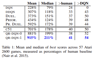
As scientific works and practice show, quantile regression is generally less affected by various outliers. This makes the model training process more stable. Moreover, the results of such training are less biased. The authors of the method presented the results of learning the work of trained models on 57 Atari games in comparison with the achievements of models trained by other algorithms. The data demonstrates that the average result is almost 4 times higher than the result of the original Q-learning (DQN). Below is a table of results from the original article [6]

Improving the model usability Previously, when creating EAs for testing all reinforcement learning models, we created various methods for choosing an action based on the feed forward results of the trained model. The creation of the new class allows us to implement methods that perform this functionality. For a greedy action selection based on the maximum expected reward, let us create the getAction method. Its algorithm is quite simple. We will only use the getResults method described above to obtain the results of the feed forward pass. From the resulting buffer, we select the element with the highest value.

int CQRDQN::getAction(void)
  {
   CBufferFloat *temp;
   getResults(temp);
   if(!temp)
      return -1;
//---
   return temp.Maximum(0, temp.Total());
  }

We do not implement the ɛ-greedy action choice strategy since it is used in the process of training the model to increase the environment learning degree. Because of our rewards policy, there is no need to use these methods. In the learning process, we provide targets for all possible agent actions.

The second getSample method will be used for a random selection of an action from the probability distribution, in which a bigger reward has a bigger probability. To eliminate unnecessary data copying between matrices and data buffers, we will partially repeat the algorithm of the getResults method.

int CQRDQN::getSample(void)
  {
   CBufferFloat* resultVals;
   CNet::getResults(resultVals);
   if(!resultVals)
      return -1;
   vectorf temp;
   if(!resultVals.GetData(temp))
     {
      delete resultVals;
      return -1;
     }
   delete resultVals;
   matrixf q;
   if(!q.Init(1, temp.Size()) || !q.Row(temp, 0) || !q.Reshape(iActions, iNumbers))
     {
      delete resultVals;
      return -1;
     }

After that, we normalize the results of the feed forward pass using the SoftMax function. These will be the action selection probabilities.

   if(!q.Mean(1).Activation(temp, AF_SOFTMAX))
      return -1;
   temp = temp.CumSum();

Let's collect the vector of cumulative totals of probabilities and implement sampling from the resulting probability distribution vector.

   int err_code;
   float random = (float)Math::MathRandomNormal(0.5, 0.5, err_code);
   if(random >= 1)
      return (int)temp.Size() - 1;
   for(int i = 0; i < (int)temp.Size(); i++)
      if(random <= temp[i] && temp[i] > 0)
         return i;
//---
   return -1;
  }

Return the sampling result to the caller program.

We have looked at feed forward and backward methods, as well as methods for obtaining the model results. But there are still a number of unanswered questions. One of them is the model update method Target Net — UpdateTarget. We referred to this method when discussing the backpropagation method. Although this method is called from another class method, I decided to make it public and give access to it to the user. True, we eliminated the need to control the Target Net state from the user side. However, we do not limit the freedom of choice. If necessary, the user can control everything.

The method algorithm is quite simple. We simply call the current object's save method first. Then, we call the data recovery method Target Net. For every operation we control the execution process. Once the Target Net is successfully updated, reset the backward iterations counter.

bool CQRDQN::UpdateTarget(string file_name)
  {
   if(!Save(file_name, 0, false))
      return false;
   float error, undefine, forecast;
   datetime time;
   if(!cTargetNet.Load(file_name, error, undefine, forecast, time, false))
      return false;
   iCountBackProp = 0;
//---
   return true;
  }

Pay attention to the difference in object classes. We work in the new CQRDQN class, while Target Net is an instance of the parent CNet class. The point is that we use only the feed forward functionality from Target Net. This method has not been modified in our class. Therefore, there should be no problem in using the parent class. At the same time, when using an instance of the CQRDQN class, for Target Net the inner Target Net object for the new instance will be recursively created. Such a recurrent process can lead to critical errors. Therefore, such an insignificant detail can have significant consequences for the operation of the entire program.

We have considered the main functionality of the new CQRDQN class which implements the quantile regression algorithm in the distributed Q-learning (QR-DQN). The method was introduced in October 2017, in the article "Distributional Reinforcement Learning with Quantile Regression".

The class also implemented methods to save the model - Save - and to restore it later - Load. The changes in these methods are not so complicated. You can study them in the code attached below. Now I propose to move on to testing the new class.

3. Testing

Let's start testing the new class by training the model. A special EA QRDQN-learning.mq5 has been created to train the model. The EA was created based on the original Q-learning Q-learning.mq5 EA. In this EA, we have changed the class of the model to be trained and have removed the Target net model instance declaration.

CSymbolInfo          Symb;
MqlRates             Rates[];
CQRDQN               StudyNet;
CBufferFloat        *TempData;
CiRSI                RSI;
CiCCI                CCI;
CiATR                ATR;
CiMACD               MACD;

In the EA initialization method, load the model from a previously created file. Forcibly turn on the learning mode of all neural layers. Define the depth of the analyzed history equal to the size of the source data layer. Input the size of the area of admissible actions into the model. Also specify the update period for Target Net. In this case, I indicated a deliberately overestimated value since I plan to control the model update process myself.

int OnInit()
  {
//---
.........
.........
//---
   if(!StudyNet.Load(FileName + ".nnw", dtStudied, false))
      return INIT_FAILED;
   if(!StudyNet.TrainMode(true))
      return INIT_FAILED;
//---
   if(!StudyNet.GetLayerOutput(0, TempData))
      return INIT_FAILED;
   HistoryBars = TempData.Total() / 12;
   if(!StudyNet.SetActions(Actions))
      return INIT_PARAMETERS_INCORRECT;
   StudyNet.SetUpdateTarget(1000000);
//---
........
//---
   return(INIT_SUCCEEDED);
  }

The model is trained in the Train function.

void Train(void)
  {
//---
   MqlDateTime start_time;
   TimeCurrent(start_time);
   start_time.year -= StudyPeriod;
   if(start_time.year <= 0)
      start_time.year = 1900;
   datetime st_time = StructToTime(start_time);

In the function, we define the training period and load the historical data. This process is completely preserved in its original form.

   int bars = CopyRates(Symb.Name(), TimeFrame, st_time, TimeCurrent(), Rates);
   if(!RSI.BufferResize(bars) || !CCI.BufferResize(bars) || !ATR.BufferResize(bars) || !MACD.BufferResize(bars))
     {
      PrintFormat("%s -> %d", __FUNCTION__, __LINE__);
      ExpertRemove();
      return;
     }
   if(!ArraySetAsSeries(Rates, true))
     {
      PrintFormat("%s -> %d", __FUNCTION__, __LINE__);
      ExpertRemove();
      return;
     }
//---
   RSI.Refresh();
   CCI.Refresh();
   ATR.Refresh();
   MACD.Refresh();

Next, we implement a system of nested loops for the model training process. The outer loop counts down the training epochs for updating the Target net model.

   int total = bars - (int)HistoryBars - 240;
   bool use_target = false;
//---
   for(int iter = 0; (iter < Iterations && !IsStopped()); iter ++)
     {
      int i = 0;
      uint ticks = GetTickCount();
      int count = 0;
      int total_max = 0;

In the nested loop, we iterate through the feed forward and backward passes. Here we will first prepare historical data to describe the two subsequent states of the system. One will be used for the feed forward pass of the model we are training. The second one will be used for Target Net.

      for(int batch = 0; batch < (Batch * UpdateTarget); batch++)
        {
         i = (int)((MathRand() * MathRand() / MathPow(32767, 2)) * total + 240);
         State1.Clear();
         State2.Clear();
         int r = i + (int)HistoryBars;
         if(r > bars)
            continue;
         for(int b = 0; b < (int)HistoryBars; b++)
           {
            int bar_t = r - b;
            float open = (float)Rates[bar_t].open;
            TimeToStruct(Rates[bar_t].time, sTime);
            float rsi = (float)RSI.Main(bar_t);
            float cci = (float)CCI.Main(bar_t);
            float atr = (float)ATR.Main(bar_t);
            float macd = (float)MACD.Main(bar_t);
            float sign = (float)MACD.Signal(bar_t);
            if(rsi == EMPTY_VALUE || cci == EMPTY_VALUE || atr == EMPTY_VALUE || macd == EMPTY_VALUE ||
               sign == EMPTY_VALUE)
               continue;
            //---
            if(!State1.Add((float)Rates[bar_t].close - open) || !State1.Add((float)Rates[bar_t].high - open) ||
               !State1.Add((float)Rates[bar_t].low - open) || !State1.Add((float)Rates[bar_t].tick_volume / 1000.0f) ||
               !State1.Add(sTime.hour) || !State1.Add(sTime.day_of_week) || !State1.Add(sTime.mon) ||
               !State1.Add(rsi) || !State1.Add(cci) || !State1.Add(atr) || !State1.Add(macd) || !State1.Add(sign))
              {
               PrintFormat("%s -> %d", __FUNCTION__, __LINE__);
               break;
              }
            if(!use_target)
               continue;
            //---
            bar_t --;
            open = (float)Rates[bar_t].open;
            TimeToStruct(Rates[bar_t].time, sTime);
            rsi = (float)RSI.Main(bar_t);
            cci = (float)CCI.Main(bar_t);
            atr = (float)ATR.Main(bar_t);
            macd = (float)MACD.Main(bar_t);
            sign = (float)MACD.Signal(bar_t);
            if(rsi == EMPTY_VALUE || cci == EMPTY_VALUE || atr == EMPTY_VALUE || macd == EMPTY_VALUE ||
               sign == EMPTY_VALUE)
               continue;
            //---
            if(!State2.Add((float)Rates[bar_t].close - open) || !State2.Add((float)Rates[bar_t].high - open) || 
               !State2.Add((float)Rates[bar_t].low - open) || !State2.Add((float)Rates[bar_t].tick_volume / 1000.0f) ||
               !State2.Add(sTime.hour) || !State2.Add(sTime.day_of_week) || !State2.Add(sTime.mon) ||
               !State2.Add(rsi) || !State2.Add(cci) || !State2.Add(atr) || !State2.Add(macd) || !State2.Add(sign))
              {
               PrintFormat("%s -> %d", __FUNCTION__, __LINE__);
               break;
              }
           }

Implement the feed forward of the model we are training.

         if(IsStopped())
           {
            PrintFormat("%s -> %d", __FUNCTION__, __LINE__);
            ExpertRemove();
            return;
           }
         if(State1.Total() < (int)HistoryBars * 12 ||
            (use_target && State2.Total() < (int)HistoryBars * 12))
            continue;
         if(!StudyNet.feedForward(GetPointer(State1), 12, true))
            return;

After that, generate a batch of rewards for all possible actions of the agent and call the feed backward method of the main model.

         Rewards.BufferInit(Actions, 0);
         double reward = Rates[i].close - Rates[i].open;
         if(reward >= 0)
           {
            if(!Rewards.Update(0, (float)(2 * reward)))
               return;
            if(!Rewards.Update(1, (float)(-5 * reward)))
               return;
            if(!Rewards.Update(2, (float) - reward))
               return;
           }
         else
           {
            if(!Rewards.Update(0, (float)(5 * reward)))
               return;
            if(!Rewards.Update(1, (float)(-2 * reward)))
               return;
            if(!Rewards.Update(2, (float)reward))
               return;
           }

Please note that in accordance with the overridden feed backward method, we input into the method not only the reward buffer, but also the current state that follows. We have also removed the block of Target Net operations and reward adjustments for the expected income of future states.

         if(!StudyNet.backProp(GetPointer(Rewards), DiscountFactor, (use_target ? GetPointer(State2) : NULL), 12, true))
            return;

Output the information about the process progress on the symbol chart.

         if(GetTickCount() - ticks > 500)
           {
            Comment(StringFormat("%.2f%%", batch * 100.0 / (double)(Batch * UpdateTarget)));
            ticks = GetTickCount();
           }
        }

This completes the nested loop operations. After completing all its iterations, we check the current model error. If the previously achieved results have been improved, save the current model state and update Target Net.

      if(StudyNet.getRecentAverageError() <= min_loss)
        {
         if(!StudyNet.UpdateTarget(FileName + ".nnw"))
            continue;
         use_target = true;
         min_loss = StudyNet.getRecentAverageError();
        }
      PrintFormat("Iteration %d, loss %.8f", iter, StudyNet.getRecentAverageError());
     }
   Comment("");
//---
   PrintFormat("%s -> %d", __FUNCTION__, __LINE__);
   ExpertRemove();
  }

This completes the operations of the outer loop and the learning function as a whole. The rest of the EA code has not changed. The full code of all classes and programs is available in the attachment.

A training model was created using the NetCreator tool. The model's architecture is the same as the architecture of the training model from the previous article. I have removed the last SoftMax normalization layer so that the model results area can replicate any results of the reward policy used.

As previously, the model was trained on EURUSD historical data, H1 timeframe. Historical data for the last 2 years was used as a training dataset.

The work of the trained model was tested in the strategy tester. A separate EA QRDQN-learning-test.mq5 was created for testing purposes. The EA was also created on the basis of similar EAs from previous articles. Its code hasn't changed much. Its full code is provided in the attachment.

In the strategy tester, the model demonstrated the ability to generate profits in a short time period of 2 weeks. More than half of the trades were closed with a profit. The average profit per trade was almost twice as large as the average loss.

Model testing graph

Model testing results

Conclusion

In this article, we got acquainted with another reinforcement learning methods. We have created a class for implementing thus method. We have trained the model and looked at its operation results in the strategy tester. Based on the results obtained, we can conclude that it is possible to use the quantile regression algorithm in distributed Q-learning to implement models which can solve real-market problems.

Once again, I would like to pay your attention to the fact that all the programs presented in the article are intended only for technology demonstration purposes. The models and the EAs require further improvement, along with the comprehensive testing, before they can be used in real trading.

References

Programs used in the article

#	Issued to	Type	Description
1	QRDQN-learning.mq5	EA	EA for optimizing the model
2	QRDQN-learning-test.mq5	EA	An Expert Advisor to test the model in the Strategy Tester
3	QRDQN.mqh	Class library	QR-DQN model class
4	NeuroNet.mqh	Class library	Library for creating neural network models
5	NeuroNet.cl	Code Base	OpenCL program code library to create neural network models
6	NetCreator.mq5	EA	Model building tool
7	NetCreatotPanel.mqh	Class library	Class library for creating the tool

Translated from Russian by MetaQuotes Ltd.
Original article: https://www.mql5.com/ru/articles/11752

Attached files |

Download ZIP

MQL5.zip (85.24 KB)

Warning: All rights to these materials are reserved by MetaQuotes Ltd. Copying or reprinting of these materials in whole or in part is prohibited.