The Box-Cox Transformation
Victor | 20 March, 2012
Introduction
While PC capacities increase, Forex traders and analysts have more possibilities for using highly developed and complex mathematical algorithms that require considerable computing resources. But the adequacy of computer resources cannot solve traders' issues alone. Efficient algorithms for analyzing market quotes are also necessary.
Currently, such areas as mathematical statistics, economics and econometrics provide a large number of methods, models and well-functioning, efficient algorithms actively used by traders for the market analysis. Most often these are standard parametric methods created with an assumption of researched sequences stability and the normality of their distribution law.
But it is not a secret that Forex quotes are sequences that can not be classified as being stable and having normal distribution law. Therefore, we cannot use "standard" parametric methods of mathematical statistics, econometrics etc. when analyzing quotes.
In the article "Box-Cox Transformation and the Illusion of Macroeconomic Series "Normality" [1] A.N. Porunov writes as follows:
"Economic analysts often have to deal with statistical data that do not pass the test for normality for one reason or another. In this situation there are two choices: either to turn to non-parametric methods that require a fair amount of mathematical training, or use special techniques that allow to convert the original "abnormal statistics" in the "normal" one, which is also quite a complex task".
Despite the fact that A.N.Porunov's quotation refers to economic analysts, it can be fully attributed to attempts to analyze the "abnormal" Forex quotes using parametric methods of mathematical statistics and econometrics. The vast majority of these methods has been developed to analyze sequences having the normal distribution law. But in most cases the fact of initial data "abnormality" is simply ignored. Besides, the mentioned methods often require not only a normal distribution, but also initial sequences stationarity.
Regression, dispersion (ANOVA) and some other types of analysis can be called "standard" methods
requiring the initial data normality. It is not possible to list all parametric methods that have limitations concerning the distribution law normality, as they occupy the whole area of, say, econometrics, except for its non-parametric methods.
To be fair, it should be added that "standard" parametric methods have different sensitivity to the deviation of the initial data distribution law from the normal value. Therefore, deviation from "normality" during the usage of such methods does not necessarily lead to disastrous consequences but, of course, it does not increase accuracy and reliability of the obtained results.
All that raises the question on the necessity of switching to non-parametric methods of analyzing and forecasting the quotes. However, parametric methods remain very attractive. This can be explained by their prevalence and sufficient amount of data, ready made algorithms and examples of their application. To use these methods properly, it is necessary to cope at least with two issues connected with initial sequences – instability and "abnormality".
Though we cannot influence the stability of initial sequences, we can try to bring their distribution law closer to the normal one. To solve this problem, there exist various transformations. The most well-known ones are briefly described in the article "The Use of Box-Cox Transformation Technique in Economic and Statistical Analyses" [2]. In this article we will consider only one of them – the Box-Cox transformation [1], [2], [3].
We should emphasize here that the use of the Box-Cox transformation, like any other transformation type, can only bring the initial sequence distribution law more or less closer to the normal one. It means that using this transformation does not guarantee that the resulting sequence will have the normal distribution law.
1. The Box-Cox Transformation
For the original sequence X of N length
![]()
The one-parameter Box-Cox transformation is found as follows:
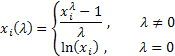
where ![]() .
.
As you can see, this transformation has only one parameter - lambda. If the lambda value is equal to zero, the logarithmic transformation of the initial sequence is carried out, in case the lambda value differs from zero, the transformation is power-law. If the lambda parameter equals to one, the initial sequence distribution law remains unchanged, though the sequence shifts, as unity is subtracted from each of its values.
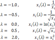
Depending on the lambda value, the Box-Cox transformation includes the following special cases:
Using the Box-Cox transformation requires all input sequence values to be positive and different from zero. If the input sequence does not satisfy these requirements, it can be moved into positive area by the volume that guarantees "positivity" of all its values.
Let's examine only the one-parameter Box-Cox transformation for now, preparing input data for it in an appropriate manner. In order to avoid negative or zero values in the input data, we will always find the lowest value of the input sequence and deduct it from each element of the sequence additionally carrying out a small shift equal to 1e-5. Such an additional shift is necessary to provide a guaranteed sequence displacement to the positive area, in case its lowest value is equal to zero.
In fact, it is not necessary to apply this displacement to "positive" sequences. But we will use the same algorithm, nevertheless, to reduce the probability of getting exceedingly big values when raising to a power during the transformation. Thus, any input sequence will be located in the positive area after the shift and have the lowest value close to zero.
Fig. 1 shows the Box-Cox transformation curves with different values of the lambda parameter. Fig. 1 has been taken from the article "Box-Cox Transformations" [3]. The horizontal grid on the chart is given on a logarithmic scale.

Fig. 1. The Box-Cox transformation in case of various values of the lambda parameter
As we can see, the "tails" of the initial distribution can be "stretched" or "pursed". The upper curve in Fig. 1 corresponds with lambda=3, while the lower one - with lambda=-2.
In order for the resulting sequence distribution law to be as close to the normal law as possible, the optimal value of the lambda parameter must be selected.
One way to determine the optimal value of this parameter is to maximize the likelihood function logarithm:
![]()
where
![]()
It means that we need to select the lambda parameter, at which this function reaches its maximum value.
The article "Box-Cox Transformations" [3] briefly deals with another way to determine the optimal value of this parameter based on searching for the highest value of the correlation coefficient between the quantiles of the normal distribution function and sorted transformed sequence. Most probably, it is possible to find some other lambda parameter optimization methods but first let's discuss searching for the likelihood function logarithm maximum mentioned earlier.
There are different ways to find it. For example, we can use a simple search. To do this, we should calculate the likelihood function value within a selected range changing the lambda parameter value in a low pitch. Also, we should select the optimal lambda parameter, at which the likelihood function has the highest value.
The pitch distance will determine the accuracy of the lambda parameter optimal value calculation. The lower the pitch, the higher the accuracy, though the required amount of calculations is proportionally increased in that case. Various algorithms of searching for the function maximum/minimum, genetic algorithms and some other methods can be used to increase calculations efficiency.
2. Transformation into the Normal Distribution Law
One of the most important tasks of the Box-Cox transformation is reduction of the input sequence distribution law to "normal" form. Let's try to find, how well such an issue can be solved with the help of this transformation.
To avoid any distraction and unnecessary repetition, we will use the algorithm of searching for the function minimum by Powell's method. This algorithm has been described in the articles "Time Series Forecasting Using Exponential Smoothing" and "Time Series Forecasting Using Exponential Smoothing (continued)".
We should create CBoxCox class for searching for the transformation parameter optimal value. In this class the above mentioned likelihood function will be realized as an objective one. PowellsMethod class [4], [5] is used as a basic one directly realizing the search algorithm.
//+------------------------------------------------------------------+
//|                                                      CBoxCox.mqh |
//|                                                    2012, victorg |
//|                                              https://www.mql5.com |
//+------------------------------------------------------------------+
#property copyright "2012, victorg"
#property link      "https://www.mql5.com"
#include "PowellsMethod.mqh"
//+------------------------------------------------------------------+
//| CBoxCox class                                                    |
//+------------------------------------------------------------------+
class CBoxCox:public PowellsMethod
  {
protected:
   double            Dat[];          // Input data
   double            BCDat[];        // Box-Cox data
   int               Dlen;          // Data size
   double            Par[1];         // Parameters
   double            LnX;            // ln(x) sum
public:
   void   CBoxCox(void) { }
   void              CalcPar(double &dat[]);
   double GetPar(int n) { return(Par[n]); }
private:
   virtual double    func(const double &p[]);
  };
//+------------------------------------------------------------------+
//| CalcPar                                                          |
//+------------------------------------------------------------------+
void CBoxCox::CalcPar(double &dat[])
  {
   int i;
   double a;
   //--- Lambda initial value
   Par[0]=1.0;
   Dlen=ArraySize(dat);
   ArrayResize(Dat,Dlen);
   ArrayResize(BCDat,Dlen);
   LnX=0;
   for(i=0;i<Dlen;i++)
     {
    //--- input data
      a=dat[i]; Dat[i]=a;
     //--- ln(x) sum
     LnX+=MathLog(a);
     }
    //--- Powell optimization
    Optimize(Par);
  }
//+------------------------------------------------------------------+
//| func                                                             |
//+------------------------------------------------------------------+
double CBoxCox::func(const double &p[])
  {
   int i;
   double a,lamb,var,mean,k,ret;

   lamb=p[0]; var=0; mean=0; k=0;
   if(lamb>5.0){k=(lamb-5.0)*400; lamb=5.0;}         // Lambda >  5.0
   else if(lamb<-5.0){k=-(lamb+5.0)*400; lamb=-5.0;} // Lambda < -5.0

   //--- Lambda != 0.0
   if(lamb!=0)
     {
      for(i=0;i<Dlen;i++)
        {
          //--- Box-Cox transformation
         BCDat[i]=(MathPow(Dat[i],lamb)-1.0)/lamb;
          //--- average value calculation
         mean+=BCDat[i]/Dlen;
        }
     }
    //--- Lambda == 0.0
    else
     {
      for(i=0;i<Dlen;i++)
        {
          //--- Box-Cox transformation
         BCDat[i]=MathLog(Dat[i]);
          //--- average value calculation
         mean+=BCDat[i]/Dlen;
        }
     }
   for(i=0;i<Dlen;i++)
     {
      a=BCDat[i]-mean;
       //--- variance
      var+=a*a/Dlen;
     }
   //--- log-likelihood
   ret=Dlen*MathLog(var)/2.0-(lamb-1)*LnX;
   return(k+ret);
  }
//------------------------------------------------------------------------------------
Now, all we have to do to find the lambda parameter optimal value is to refer to the CalcPar method of the mentioned class by providing it with the link to the array containing the input data. We can get the obtained parameter optimal value by referring to GetPar method. As it has been said before, the input data must be positive.
PowellsMethod class implements the algorithm of searching for the minimum of the function of lots of variables, but in our case only a single parameter is optimized. That leads to the fact that Par[] array dimension is equal to one. It means that the array contains only one value. Theoretically we can use a standard variable instead of the parameters array in this case but this would require implementing changes into the PowellsMethod basic class code. Presumably, there will not be any issues, if we compile the source MQL5 code using the arrays containing only one element.
We should mind the fact that CBoxCox::func() function contains a limitation of the range of the lambda parameter permissible values. In our case, this range is limited to values from -5 to 5. This is done in order to avoid getting exceedingly big or too small values when raising the input data to the lambda degree.
Besides, if we get exceedingly big or too small lambda values during the optimization, this may indicate that the sequence is of little use for the selected transformation type. Therefore, it would be wise in any case not to exceed some reasonable range when calculating the lambda value.
3. Random Sequences
Let's write a test script that will carry out the Box-Cox transformation of the pseudorandom sequence formed by us using CBoxCox class.
Below is the source code of such a script.
//+------------------------------------------------------------------+
//|                                                  BoxCoxTest1.mq5 |
//|                                                    2012, victorg |
//|                                              https://www.mql5.com |
//+------------------------------------------------------------------+
#property copyright "2012, victorg"
#property link      "https://www.mql5.com"
#include  "CBoxCox.mqh"
#include  "RNDXor128.mqh"
CBoxCox   Bc;
RNDXor128 Rnd;
//+------------------------------------------------------------------+
//| Script program start function                                    |
//+------------------------------------------------------------------+
void OnStart()
  {
   int i,n;
   double dat[],bcdat[],lambda,min;
//--- data size
   n=1600;
//--- input array preparation
   ArrayResize(dat,n);
//--- transformed data array
   ArrayResize(bcdat,n);
   Rnd.Reset();
//--- random sequence generation
   for(i=0;i<n;i++)dat[i]=Rnd.Rand_Exp();

//--- input data shift
   min=dat[ArrayMinimum(dat)]-1e-5;

   for(i=0;i<n;i++)dat[i]=dat[i]-min;

//--- optimization by lambda
   Bc.CalcPar(dat);
   lambda=Bc.GetPar(0);
   PrintFormat("Iterations= %i,   lambda= %.4f",Bc.GetIter(),lambda);

   if(lambda!=0){for(i=0;i<n;i++)bcdat[i]=(MathPow(dat[i],lambda)-1.0)/lambda;}
   else         {for(i=0;i<n;i++)bcdat[i]=MathLog(dat[i]);}     // Lambda == 0.0

//--- dat[]   <-- input data
//--- bcdat[] <-- transformed data
  }
//-----------------------------------------------------------------------------------
A pseudorandom sequence with the exponential law of distribution is used as the input transformed data in the shown script. The sequence length is set in n variable and is equal to 1600 values in this case.
RNDXor128 class (George Marsaglia, Xorshift RNG) is used for generation of a pseudorandom sequence. This class was described in the article "Analysis of the Main Characteristics of Time Series" [6]. All files necessary for BoxCoxTest1.mq5 script compilation are in the Box-Cox-Tranformation_MQL5.zip archive. These files must be located in one directory for successful compilation.
When the shown script is executed, the input sequence is formed, moved to the positive values area and searching for the lambda parameter optimal value is performed. Then the message containing the obtained lambda value and the number of the searching algorithm passes are displayed. Transformed sequence will be created in the bcdat[] output array as a result.
This script in its current form allows only to prepare the transformed sequence for its further use and does not implement any changes. When writing this article, the analysis type described in the article "Analysis of the Main Characteristics of Time Series" [6] has been selected for evaluation of the transformation results. The scripts used for that are not shown in this article to reduce the volume of published codes. Only ready made analysis graphical results are presented below.
Fig. 2 shows the histogram and the chart provided by the normal distribution scale for the pseudorandom sequence with the exponential distribution law used in the BoxCoxTest1.mq5 script. Jarque-Bera test result JB=3241.73, p= 0.000. As we can see, the input sequence is not "normal" at all and, as expected, its distribution is similar to the exponential one.

Fig. 2. Pseudorandom sequence with the exponential distribution law. Jarque-Bera test JB=3241.73, р=0.000.

Fig. 3. Transformed sequence. Lambda parameter=0.2779, Jarque-Bera test JB=4.73, р=0.094
Fig. 3 shows the result of the transformed sequence analysis
(BoxCoxTest1.mq5 script, bcdat[] array). Transformed sequence distribution law is much more closer to the normal one, which is also
confirmed by Jarque-Bera test results JB=4.73, p=0.094. The obtained lambda parameter value=0.2779.
The Box-Cox transformation has proved itself to be suitable enough in this example. It seems that the resulting sequence has become much closer to the "normal" one and Jarque-Bera test result has decreased from JB=3241.73 to JB=4.73. It is not surprising, since the chosen sequence evidently fits this type of transformation quite well.
Let's examine another example of the Box-Cox transformation of the pseudorandom sequence. We should create a "suitable" input sequence for the Box-Cox transformation considering its power-law nature. To achieve this, we need to generate a pseudorandom sequence (that already has the distribution law close to the normal one) and then distort it by raising all of its values to the power of 0.35. We can expect that the Box-Cox transformation will return the original normal distribution to the input sequence with great precision.
Below is the source code of BoxCoxTest2.mq5 text script.
This script differs from the previous one only by the fact that another input sequence is generated in it.
//+------------------------------------------------------------------+
//|                                                  BoxCoxTest2.mq5 |
//|                                                    2012, victorg |
//|                                              https://www.mql5.com |
//+------------------------------------------------------------------+
#property copyright "2012, victorg"
#property link      "https://www.mql5.com"
#include  "CBoxCox.mqh"
#include  "RNDXor128.mqh"
CBoxCox   Bc;
RNDXor128 Rnd;
//+------------------------------------------------------------------+
//| Script program start function                                    |
//+------------------------------------------------------------------+
void OnStart()
  {
   int i,n;
   double dat[],bcdat[],lambda,min;
//--- data size
   n=1600;
//--- input data array
   ArrayResize(dat,n);
//--- transformed data array
   ArrayResize(bcdat,n);
   Rnd.Reset();
//--- random sequence generation
   for(i=0;i<n;i++)dat[i]=Rnd.Rand_Norm();

//--- input data shift
   min=dat[ArrayMinimum(dat)]-1e-5;

   for(i=0;i<n;i++)dat[i]=dat[i]-min;
   for(i=0;i<n;i++)dat[i]=MathPow(dat[i],0.35);

//--- optimization by lambda
   Bc.CalcPar(dat);
   lambda=Bc.GetPar(0);

   PrintFormat("Iterations= %i,   lambda= %.4f",Bc.GetIter(),lambda);

   if(lambda!=0) { for(i=0;i<n;i++)bcdat[i]=(MathPow(dat[i],lambda)-1.0)/lambda;   }
   else          { for(i=0;i<n;i++)bcdat[i]=MathLog(dat[i]);  }     // Lambda == 0.0

//-- dat[]   <-- input data
//-- bcdat[] <-- transformed data
  }
//-----------------------------------------------------------------------------------
The input pseudorandom sequence with the normal distribution law is generated in the shown script. It is shifted to the positive values area and then all elements of this sequence are raised to the power of 0.35. After completion of the script operation dat[] array contains the input sequence, while bcdat[] array contains the transformed one.
Fig. 4 shows the characteristics of the input sequence that has lost its original normal distribution because of raising to the power of 0.35. In that case Jarque-Bera test shows JB=3609.29, p= 0.000.

Fig. 4. Input pseudorandom sequence. Jarque-Bera test JB=3609.29, p=0.000.

Fig. 5. Transformed sequence. Lambda parameter=2.9067, Jarque-Bera test JB=0.30, p=0.859
As shown in Fig. 5, the transformed sequence has the distribution law close enough to the normal one, which is also confirmed by Jarque-Bera test value JB=0.30, p=0.859.
These examples of the Box-Cox transformation use have demonstrated very good results. But we should not forget that in both cases we have dealt with the sequences that were most convenient for this transformation. Therefore, these results can be viewed simply as a confirmation of the performance of the algorithm we have created.
4. Quotes
After we have confirmed the normal performance of the algorithm implementing the Box-Cox transformation, we should try applying it to real Forex quotes, as we want to reduce them to the normal distribution law.
We will use the sequences that were described in the article "Time Series Forecasting Using Exponential Smoothing (continued)" [5] as test quotes. They are placed in the \Dataset2 directory of the Box-Cox-Tranformation_MQL5.zip archive and provide real quotes, 1200 values of which have been saved to the appropriate files. Extracted \Dataset2 folder must be placed to \MQL5\Files directory of the terminal to provide access to these files.
Let's assume that these quotes are not stationary sequences. Therefore, we will not extend the analysis results to the so-called general population, but only consider them as characteristics of this particular finite length sequence.
Besides, it should be mentioned again that if there is no stationarity, different quotes fragments of the same currency pair follow widely different distribution laws.
Let's create a script allowing to read sequence values from a file and perform its Box-Cox transformation. From the test scripts shown above it will differ only in the way of the input sequence forming. Below is the source code of such a script, while the BoxCoxTest3.mq5 script is placed in the attached archive.
//+------------------------------------------------------------------+
//|                                                  BoxCoxTest3.mq5 |
//|                                                    2012, victorg |
//|                                              https://www.mql5.com |
//+------------------------------------------------------------------+
#property copyright "2012, victorg"
#property link      "https://www.mql5.com"
#include  "CBoxCox.mqh"
CBoxCox   Bc;
//+------------------------------------------------------------------+
//| Script program start function                                    |
//+------------------------------------------------------------------+
void OnStart()
  {
   int i,n;
   double dat[],bcdat[],lambda,min;
   string fname;
//--- input data file
   fname="Dataset2\\EURUSD_M1_1200.txt";
//--- data reading
   if(readCSV(fname,dat)<0){Print("Error."); return;}
//--- data size
   n=ArraySize(dat);
//--- transformed data array
   ArrayResize(bcdat,n);

//--- input data array
   min=dat[ArrayMinimum(dat)]-1e-5;
   for(i=0;i<n;i++)dat[i]=dat[i]-min;

//--- lambda parameter optimization
   Bc.CalcPar(dat);
   lambda=Bc.GetPar(0);
   PrintFormat("Iterations= %i,   lambda= %.4f",Bc.GetIter(),lambda);

   if(lambda!=0){for(i=0;i<n;i++)bcdat[i]=(MathPow(dat[i],lambda)-1.0)/lambda;}
   else         {for(i=0;i<n;i++)bcdat[i]=MathLog(dat[i]);}     // Lambda == 0.0

//--- dat[]   <-- input data
//--- bcdat[] <-- transformed data
  }
//+------------------------------------------------------------------+
//| readCSV                                                          |
//+------------------------------------------------------------------+
int readCSV(string fnam,double &dat[])
  {
   int n,asize,fhand;

   fhand=FileOpen(fnam,FILE_READ|FILE_CSV|FILE_ANSI);
   if(fhand==INVALID_HANDLE)
     {
      Print("FileOpen Error!");
      return(-1);
     }
   asize=512;
   ArrayResize(dat,asize);
   n=0;
   while(FileIsEnding(fhand)!=true)
     {
      dat[n++]=FileReadNumber(fhand);
      if(n+128>asize)
        {
         asize+=128;
         ArrayResize(dat,asize);
        }
     }
   FileClose(fhand);
   ArrayResize(dat,n-1);
   return(0);
  }
//-----------------------------------------------------------------------------------
All values (there are 1200 of them in our case) are imported to the dat[] array in this script from the quotes file, the name of which is set in the fname variable. Further on, the shift of the initial sequence, searching for the optimal parameter value and the Box-Cox transformation are performed, in the way it was described above. After the script has been executed, transformation result is located in the bcdat[] array.
As can be seen from the shown source code, EURUSD M1 quotes sequence has been selected in the script for the transformation. Original and transformed sequence analysis result is shown in Fig. 6 and 7.

Fig. 6. EURUSD M1 input sequence. Jarque-Bera test JB=100.94, p=0.000.

Fig. 7. Transformed sequence. Lambda parameter=0.4146, Jarque-Bera test JB=39.30, p=0.000
According to the characteristics shown in Fig. 7, the result of EURUSD M1 quotes transformation is not as impressive, as pseudorandom sequences transformation results shown earlier. The Box-Cox transformation is not able to cope with all types of input sequences, though it is considered to be universal enough. For example, it is impracticable to expect from the power-law transformation to turn the two-topped distribution into the normal one.
Although the distribution law shown in Fig. 7 can hardly be considered normal, we still can see a considerable decrease of Jarque-Bera test values like in previous examples. While JB=100.94 for the original sequence, it shows JB=39.30 after the transformation. It means that the distribution law has managed to approach the normal values to some extent after the transformation.
Approximately the same results have been obtained when transforming different fragments of other quotes. Every time the Box-Cox transformation brought the distribution law closer to the normal one to a greater or lesser extent. However, it never became normal.
A series of experiments with various quotes transformation allows to draw the quite expectable conclusion – the Box-Cox transformation allows to bring Forex quotes distribution law close to the normal one, but it cannot guarantee reaching the true normality of the transformed data distribution law.
Is it reasonable to carry out the transformation, which still does not bring the original sequence to the normal one? There is no definite answer to this question. In each specific case we should take an individual decision concerning the need for the Box-Cox transformation. In this case much will depend on the type of parametric methods that are used in the quotes analysis and sensibility of these methods to the deviation of the initial data from the normal distribution law.
5. Trend Removal
The upper part of Fig. 6 displays the chart of the EURUSD M1 original sequence used in the BCTransform.mq5 script. It can be easily seen that its values are increasing almost uniformly all along the sequence. At a first approximation, we can conclude that the sequence contains the linear trend. Presence of such "trendiness" suggests that we should try to exclude the trend before carrying out various transformations and analyzing the received sequence.
Removal of a trend from the analyzed input sequences probably should not be considered as a method suitable for absolutely all cases. But let's suppose that we are going to analyze the sequence shown in Fig. 6 to find periodic (or cyclic) components in it. In this case we surely can subtract the linear trend from the input sequence after defining trend's parameters.
Removal of a linear trend will not affect the detection of periodic components. It even may be useful and make the results of such analysis more accurate or reliable to some degree depending on the selected analysis method.
If we decided that a trend removal may be useful in some cases, then it probably makes sense to examine, how the Box-Cox transformation copes with a sequence after a trend has been excluded from it.
In any situation, when removing a trend we will have to decide, what curve should be used for the trend approximation? This can be a straight line, curves of the higher order, moving averages etc. In this case, let's choose, if I may say so, the extreme version in order not to be distracted by the optimal curve selection issue. We will use the increments of the original sequence, i.e. the differences between its current and previous values instead of the original sequence itself.
As soon as we discussing the increments analysis, it is impossible not to comment on some related points.
In various articles and forums the necessity of transition to increments analysis is justified in such a way that it can leave the wrong impression about the properties of such a transition. Transition to increments analysis is often described as a sort of transformation that is able to turn an original sequence into a stationary one or normalize its distribution law. But is it true? Let's try to answer this question.
We should begin from the fact that the essence of transition to increments analysis is comprised of a very simple idea of dividing an original sequence into two components. We can demonstrate that as follows.
Assume that we have the input sequence
![]()
And we have decided to divide it for whatever reasons into a trend and some remaining elements that appeared after the subtraction of the
trend values from the original sequence elements. Suppose that we have decided to use a simple moving average with a smoothing period equal to two sequence elements for a trend approximation.
Such a moving average can be calculated as the sum of two adjacent sequence elements divided by two. In that case the residue from the subtraction of the average from the original sequence will be equal to the difference between the same adjacent elements divided by two.
Let's denote the above mentioned average value as S, while the residue will be D. In case we move the permanent factor 2 to the left part of the equation for more clarity, we will get as follows:
![]()
After completing our fairly simple transformations, we have divided our original sequence into two components, one of which is the sum of the adjacent sequences values, and the other consists of the differences. These are exactly the sequences we call increments, while the sums form the trend.
In this regard, it would be more reasonable to consider the increments as some part of the original sequence. Therefore, we should not forget that, if we switch to the increments analysis, then the other part of the sequence defined by the sums is often simply disregarded, unless we do not analyze it separately, of course.
The easiest way to get an idea of what sort of benefits we can receive with this division of the sequence is to apply the spectral method.
Directly from the expressions given above we can derive that S component is a result of the original sequence filtration with the use of the low frequency filter having the impulse characteristics h=1.1. Accordingly, D component is a result of the filtration with the use of the high frequency filter having the impulse characteristics h=-1.1. Fig. 8 nominally displays frequency characteristics of such filters.

Fig. 8. Amplitude-frequency characteristics
Suppose that we have moved from the direct analysis of the sequence itself to the analysis of its differences. What can we expect here? There are various options in that case. We will have a brief look only at some of them.
- In case the basic energy of the analyzed process is concentrated in the low-frequency region of the original sequence, transition to the differences analysis will just suppress that energy, making it more complex or even impossible to continue the analysis;
- In case the basic energy of the analyzed process is concentrated in the high-frequency region of the original sequence, transition to the differences analysis may lead to positive effects because of the filtration of the interfering low-frequency components. But this is possible, only in case such a filtration will not significantly affect the properties of the analyzed process;
- We can also mention the case when the energy of the analyzed process is uniformly distributed all over the sequence frequency range. In that case we will irreversibly distort the process after the transition to the analysis of its differences by suppressing its low-frequency part.
Similarly we can draw conclusions about the results of the transition to the differences analysis for any other trend combinations, short-term trend, interfering noise and so on. But in any case, the transition to the differences analysis will not lead to a stationary form of the analyzed process and will not normalize the distribution process.
Based on the above said, we can conclude that a sequence does not "improve" automatically after transition to the differences analysis. We can assume that in some cases it is better to analyze both the input sequence and the differences together with the sums of its adjacent values to receive more clear knowledge of the input sequence, while the final conclusions about the properties of this sequence should be made based on the joint review of all obtained results.
Let's get back to the subject of our article and see how the Box-Cox transformation behaves in case of the transition to the increments analysis of the EURUSD M1 sequence shown in Fig.6. To do this, we will use the BoxCoxTest3.mq5 script shown earlier, in which we will replace the sequence values with differences (increments) after computing these sequence values from the file. Since no other changes to the script source code are implemented, there is no point in publishing it. We will just show the results of its functioning analysis instead.

Fig. 9. EURUSD M1 increments. Jarque-Bera test JB=32494.8, p=0.000

Fig. 10. Transformed sequence. Lambda parameter=0.6662, Jarque-Bera test JB=10302.5, p=0.000
Fig. 9 shows the characteristics of the sequence consisting of EURUSD M1 increments (differences), while Fig. 10 shows its characteristics obtained after the Box-Cox transformation. Despite the fact that the Jarque-Bera test value has decreased by more than three times from JB = 32494.8 to JB = 10302.5 after the transformation, the transformed sequence distribution law is still far from normal.
However, we should not jump to hasty conclusions thinking that the Box-Cox transformation cannot cope with the increments transformation properly. We have considered only a special case. Dealing with other input sequences, we may obtain completely different results.
6. Cited Examples
All previously cited examples of the Box-Cox transformation relate to the case when the original sequence distribution law is supposed to be reduced to the normal one or, perhaps, to the law that is as close to the normal one as possible. As it has been mentioned at the beginning, such transformation can be necessary when using the parametric analysis methods, which can be quite sensitive to the deviation of an examined sequence distribution law from the normal one.
Shown examples have demonstrated that in all cases after the transformation, according to Jarque-Bera test results, we have actually received the sequences having the distribution law being closer to the normal one comparing with the original sequences. This fact clearly shows the versatility and efficiency of the Box-Cox transformation.
But we should not overestimate the possibilities of the Box-Cox transformation and assume that any input sequence will be transformed into a strictly normal one. As can be seen from the above examples, this is far from true. Neither original, nor transformed sequence cannot be considered normal for actual quotes.
The Box-Cox transformation has been considered only in its more visual, one-parameter form, so far. This has been done to simplify the first encounter with it. This approach is justified to demonstrate the capabilities of this transformation, but for practical purposes it would probably be better to use a more general form of its presentation.
7. The General Form of the Box-Cox Transformation
It should be recalled that the Box-Cox transformation is applicable only to the sequences having positive and non-zero values. In practice this requirement is easily satisfied by a simple shift of a sequence to the positive area but the magnitude of the shift within the positive area can have a direct impact on the transformation result.
Therefore, the shift value can be regarded as an additional transformation parameter and optimize it along with the lambda parameter, not allowing the sequence values to enter the negative area.
For the original sequence X of N length:
![]()
the expressions determining more general form of the two-parameter Box-Cox transformation are the following ones:
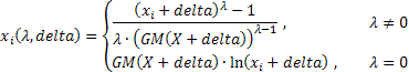
where:
![]() ;
;
GM() - geometric mean.
The geometric mean of the sequence can be calculated the following way:
![]()
As we can see, two parameters are already used in the shown expressions - lambda and delta. Now, we have to optimize both of these parameters simultaneously during the transformation. Despite the slight complication of the algorithm, the introduction of an additional parameter may certainly increase the transformation efficiency. Besides, the additional normalizing factors have appeared in the expressions compared with the previously used transformation. With this factors the transformation result will retain its dimension during the lambda parameter alteration.
More information on the Box-Cox transformation can be found in [7], [8]. Some other transformations of the same type are briefly described in [8].
Here are the main features of the present, more general transformation form:
- The transformation itself requires from the input sequence to contain only positive values. Inclusion of the additional delta parameter allows to automatically perform the required shift of the sequence when fulfilling some definite conditions;
- When selecting the delta parameter optimal value, its magnitude must guarantee "positivity" of all sequence values;
- The transformation is continuous in case of the lambda parameter alteration including the changes near its zero value;
- Transformation result retains its dimension in case of the alteration of the lambda parameter value.
The likelihood function logarithm criterion was used in all previously cited examples when searching for the lambda parameter optimal value. Of course, this is not the only way to estimate the optimal value of the transformation parameters.
As an example, we can mention the method of the parameters optimization, at which the maximum value of the correlation coefficient between a transformed sequence sorted in an ascending manner and a sequence of the normal distribution function quantiles is searched for. This variant has previously been mentioned in the article. The values of the normal distribution function quantiles can be calculated according to the expressions suggested by James J. Filliben [9].
The expressions that determine the general form of the two-parameter transformation are certainly more cumbersome than previously considered ones. Perhaps, that is the reason of the fact that such type of transformation is used quite rarely in mathematical and statistical packages. Cited expressions have been realized in MQL5 to have the possibility to use the Box-Cox transformation in more general form if necessary.
CFullBoxCox.mqh file contains the source code of the CFullBoxCox class that performs the search for the optimal value of the transformation parameters. As it has already been mentioned, the optimization process is based on the calculation of the correlation coefficient.
//+------------------------------------------------------------------+
//|                                                  CFullBoxCox.mqh |
//|                                                    2012, victorg |
//|                                              https://www.mql5.com |
//+------------------------------------------------------------------+

#property copyright "2012, victorg"
#property link      "https://www.mql5.com"

#include "PowellsMethod.mqh"
//+------------------------------------------------------------------+
//| CFullBoxCox class                                                |
//+------------------------------------------------------------------+
class CFullBoxCox:public PowellsMethod
  {
protected:
  int    Dlen;                     // data size
  double Dat[];                    // input data array
  double Shift[];                  // input data array with the shift
  double BCDat[];                  // transformed data (Box-Cox)
  double Mean;                     // transformed data average value
  double Cdf[];                    // Quantile of the distribution cumulative function
  double Scdf;                     // Square root of summ of Quantile^2
  double R;                        // correlation coefficient
  double DeltaMin;                 // Delta minimum value
  double DeltaMax;                 // Delta maximum value
  double Par[2];                   // parameters array
public:
  void   CFullBoxCox(void)       { }
  void   CalcPar(double &dat[]);
  double GetPar(int n)           { return(Par[n]); }
private:
  double ndtri(double y0);         // the function opposite to the normal distribution function
  virtual double func(const double &p[]);
  };
//+------------------------------------------------------------------+
//| CalcPar                                                          |
//+------------------------------------------------------------------+
void CFullBoxCox::CalcPar(double &dat[])
  {
  int i;
  double a,max,min;

  Dlen=ArraySize(dat);
  ArrayResize(Dat,Dlen);
  ArrayResize(Shift,Dlen);
  ArrayResize(BCDat,Dlen);
  ArrayResize(Cdf,Dlen);
//--- copy the input data array
  ArrayCopy(Dat,dat);

  Scdf=0;
  a=MathPow(0.5,1.0/Dlen);
  Cdf[Dlen-1]=ndtri(a); Scdf+=Cdf[Dlen-1]*Cdf[Dlen-1];
  Cdf[0]=ndtri(1.0-a); Scdf+=Cdf[0]*Cdf[0];
  a=Dlen+0.365;
  for(i=1;i<(Dlen-1);i++)
    {
    //--- calculation of the distribution cumulative function Quantile
    Cdf[i]=ndtri((i+0.6825)/a);
    //--- calculation of the sum of Quantile^2
    Scdf+=Cdf[i]*Cdf[i];
    }

//--- square root of the sum of Quantile^2
  Scdf=MathSqrt(Scdf);

  min=dat[0]; max=min;
  for(i=0;i<Dlen;i++)
    {
//--- copy the input data
    a=dat[i]; Dat[i]=a;
    if(min>a)min=a;
    if(max<a)max=a;
    }

//--- Delta minimum value
  DeltaMin=1e-5-min;
//--- Delta maximum value
  DeltaMax=(max-min)*200-min;
//--- Lambda initial value
  Par[0]=1.0;
//--- Delta initial value
  Par[1]=(max-min)/2-min;
//--- optimization using Powell method
  Optimize(Par);
  }
//+------------------------------------------------------------------+
//| func                                                             |
//+------------------------------------------------------------------+
double CFullBoxCox::func(const double &p[])
  {
  int i;
  double a,b,c,lam,del,k1,k2,gm,gmpow,mean,ret;

  lam=p[0]; del=p[1]; k1=0; k2=0;
  if (lam>5.0){k1=(lam-5.0)*400; lam=5.0;}                    // Lambda >  5.0
  else if(lam<-5.0){k1=-(lam+5.0)*400; lam=-5.0;}             // Lambda < -5.0
  if (del>DeltaMax){k2=(del-DeltaMax)*400; del=DeltaMax;}    // Delta > DeltaMax
  else if(del<DeltaMin){k2=(DeltaMin-del)*400; del=DeltaMin; // Delta < DeltaMin

  gm=0;
  for(i=0;i<Dlen;i++)
    {
    Shift[i]=Dat[i]+del;
    gm+=MathLog(Shift[i]);
    }

//--- geometric mean
  gm=MathExp(gm/Dlen);
  gmpow=lam*MathPow(gm,lam-1);
  mean=0;
//--- Lambda != 0.0
   if(lam!=0)
    {
    for(i=0;i<Dlen;i++)
      {
      a=(MathPow(Shift[i],lam)-1.0)/gmpow;
       //--- transformed data (Box-Cox)
      BCDat[i]=a;
       //--- average value
      mean+=a;
      }
    }
  //--- Lambda == 0.0
  else
     {
    for(i=0;i<Dlen;i++)
      {
      a=gm*MathLog(Shift[i]);
       //--- transformed data (Box-Cox)
      BCDat[i]=a;
      //--- average value
      mean+=a;
      }
    }
  mean=mean/Dlen;
  //--- sorting of the transformed data array
  ArraySort(BCDat);
  a=0; b=0;
  for(i=0;i<Dlen;i++)
    {
    c=(BCDat[i]-mean);
    a+=Cdf[i]*c;
    b+=c*c;
    }
  //--- correlation coefficient
  ret=a/(Scdf*MathSqrt(b));
  return(k1+k2-ret);
  }
//+------------------------------------------------------------------+
//| The function opposite to the normal distribution function        |
//| Prototype:                                                       |
//| Cephes Math Library Release 2.8: June, 2000                      |
//| Copyright 1984, 1987, 1989, 2000 by Stephen L. Moshier           |
//+------------------------------------------------------------------+
double CFullBoxCox::ndtri(double y0)
  {
  static double s2pi =2.50662827463100050242E0; // sqrt(2pi)
  static double P0[5]={-5.99633501014107895267E1,  9.80010754185999661536E1,
                       -5.66762857469070293439E1,  1.39312609387279679503E1,
                       -1.23916583867381258016E0};
  static double Q0[8]={ 1.95448858338141759834E0,  4.67627912898881538453E0,
                        8.63602421390890590575E1, -2.25462687854119370527E2,
                        2.00260212380060660359E2, -8.20372256168333339912E1,
                        1.59056225126211695515E1, -1.18331621121330003142E0};
  static double P1[9]={ 4.05544892305962419923E0,  3.15251094599893866154E1,
                        5.71628192246421288162E1,  4.40805073893200834700E1,
                        1.46849561928858024014E1,  2.18663306850790267539E0,
                       -1.40256079171354495875E-1,-3.50424626827848203418E-2,
                       -8.57456785154685413611E-4};
  static double Q1[8]={ 1.57799883256466749731E1,  4.53907635128879210584E1,
                        4.13172038254672030440E1,  1.50425385692907503408E1,
                        2.50464946208309415979E0, -1.42182922854787788574E-1,
                       -3.80806407691578277194E-2,-9.33259480895457427372E-4};
  static double P2[9]={ 3.23774891776946035970E0,  6.91522889068984211695E0,
                        3.93881025292474443415E0,  1.33303460815807542389E0,
                        2.01485389549179081538E-1, 1.23716634817820021358E-2,
                        3.01581553508235416007E-4, 2.65806974686737550832E-6,
                        6.23974539184983293730E-9};
  static double Q2[8]={ 6.02427039364742014255E0,  3.67983563856160859403E0,
                        1.37702099489081330271E0,  2.16236993594496635890E-1,
                        1.34204006088543189037E-2, 3.28014464682127739104E-4,
                        2.89247864745380683936E-6, 6.79019408009981274425E-9};
  double x,y,z,y2,x0,x1,a,b;
  int i,code;
  if(y0<=0.0){Print("Function ndtri() error!"); return(-DBL_MAX);}
  if(y0>=1.0){Print("Function ndtri() error!"); return(DBL_MAX);}
  code=1; y=y0;
  if(y>(1.0-0.13533528323661269189)){y=1.0-y; code=0;}  // 0.135... = exp(-2)
  if(y>0.13533528323661269189)                         // 0.135... = exp(-2)
    {
    y=y-0.5;
    y2=y*y;
    a=P0[0]; for(i=1;i<5;i++)a=a*y2+P0[i];
    b=y2+Q0[0]; for(i=1;i<8;i++)b=b*y2+Q0[i];
    x=y+y*(y2*a/b);
    x=x*s2pi;
    return(x);
    }
  x=MathSqrt(-2.0*MathLog(y));
  x0=x-MathLog(x)/x;
  z=1.0/x;
//--- y > exp(-32) = 1.2664165549e-14
  if(x<8.0)
    {
    a=P1[0]; for(i=1;i<9;i++)a=a*z+P1[i];
    b=z+Q1[0]; for(i=1;i<8;i++)b=b*z+Q1[i];
    x1=z*a/b;
    }
  else
    {
    a=P2[0]; for(i=1;i<9;i++)a=a*z+P2[i];
    b=z+Q2[0]; for(i=1;i<8;i++)b=b*z+Q2[i];
    x1=z*a/b;
    }
  x=x0-x1;
  if(code!=0)x=-x;
  return(x);
  }
//------------------------------------------------------------------------------------
Some limitations are applied to the transformation parameters alteration range during the optimization. The lambda parameter value is limited by values 5.0 and -5.0. Limitations for the delta parameters are specified relative to the minimum value of the input sequence. This parameter is limited by DeltaMin=(0.00001-min) and DeltaMax=(max-min)*200-min values, where min and max are the minimum and maximum values of the input sequence elements.
FullBoxCoxTest.mq5 script demonstrates the use of the CFullBoxCox class. The source code of this script is shown below.
//+------------------------------------------------------------------+
//|                                               FullBoxCoxTest.mq5 |
//|                                                    2012, victorg |
//|                                              https://www.mql5.com |
//+------------------------------------------------------------------+
#property copyright "2012, victorg"
#property link      "https://www.mql5.com"

#include  "CFullBoxCox.mqh"
CFullBoxCox   Bc;
//+------------------------------------------------------------------+
//| Script program start function                                    |
//+------------------------------------------------------------------+
void OnStart()
  {
   int i,n;
   double dat[],shift[],bcdat[],lambda,delta,gm,gmpow;
   string fname;

//--- input file name
   fname="Dataset2\\EURUSD_M1_1200.txt";
//--- reading the data
   if(readCSV(fname,dat)<0){Print("Error."); return;}
//--- data size
   n=ArraySize(dat);
//--- shifted input data array
   ArrayResize(shift,n);
//--- transformed data array
   ArrayResize(bcdat,n);

//--- lambda and delta parameters optimization
   Bc.CalcPar(dat);
   lambda=Bc.GetPar(0);
   delta=Bc.GetPar(1);

   PrintFormat("Iterations= %i,   lambda= %.4f,   delta= %.4f",
               Bc.GetIter(),lambda,delta);
   gm=0;
   for(i=0;i<n;i++)
     {
      shift[i]=dat[i]+delta;
      gm+=MathLog(shift[i]);
     }
//--- geometric mean
   gm=MathExp(gm/n);
   gmpow=lambda*MathPow(gm,lambda-1);
   if(lambda!=0){for(i=0;i<n;i++)bcdat[i]=(MathPow(shift[i],lambda)-1.0)/gmpow;}
   else         {for(i=0;i<n;i++)bcdat[i]=gm*MathLog(shift[i]);}
//--- dat[]   <-- input data
//--- shift[] <-- input data with the shift
//--- bcdat[] <-- transformed data
  }
//+------------------------------------------------------------------+
//| readCSV                                                          |
//+------------------------------------------------------------------+
int readCSV(string fnam,double &dat[])
  {
   int n,asize,fhand;

   fhand=FileOpen(fnam,FILE_READ|FILE_CSV|FILE_ANSI);
   if(fhand==INVALID_HANDLE)
     {
      Print("FileOpen Error!");
      return(-1);
     }
   asize=512;
   ArrayResize(dat,asize);
   n=0;
   while(FileIsEnding(fhand)!=true)
     {
      dat[n++]=FileReadNumber(fhand);
      if(n+128>asize)
        {
         asize+=128;
         ArrayResize(dat,asize);
        }
     }
   FileClose(fhand);
   ArrayResize(dat,n-1);
   return(0);
  }
//------------------------------------------------------------------------------------
The input sequence is uploaded to the dat[] array from the file at the beginning of the script and then the search for the optimal values of the transformation parameters is carried out. Then the transformation itself is carried out with the use of the obtained parameters. As a result, the dat[] array contains the original sequence, the shift[] array contains the original sequence shifted by the delta value and the bcdat[] array contains the result of the Box-Cox transformation.
All files necessary for the FullBoxCoxTest.mq5 script compilation are located in the Box-Cox-Tranformation_MQL5.zip archive.
Transformation of the test sequences that we use is performed with the help of the FullBoxCoxTest.mq5 script. As it has been expected, during the analysis of the obtained data we can conclude that this two-parameter transformation type shows somewhat better results comparing with the one-parameter type. For example, for EURUSD M1 sequence, the analysis results of which are shown in Fig. 6, Jarque-Bera test value comprised JB=100.94. JB=39.30 after the one-parameter transformation (see Fig. 7), but after the two-parameter transformation (FullBoxCoxTest.mq5 script) this value went down to JB=37.49.
Conclusion
In this article we have examined the cases when the Box-Cox transformation parameters optimized so that the resulting sequence distribution law was as close to the normal one as possible. But in practice, the cases can occur when the Box-Cox transformation should be used in a slightly different way. For example, the following algorithm can be used when forecasting the time sequences:
- Preliminary values of the Box-Cox transformation parameters values and forecast models are selected;
- The Box-Cox transformation of the input data is performed;
- The forecast is carried out according to the current parameters;
- Reverse Box-Cox Transformation is carried out for the forecast results;
- The forecast error is evaluated by the input untransformed sequence;
- Parameters values are changed to minimize the forecast error and the algorithm returns to step 2.
In the algorithm above the transformation parameters are to be minimized, as well as the forecast model ones, by the forecast error minimum criterion. In this case, the Box-Cox transformation's objective is already not the transformation of the input sequence into the normal distribution law.
Now, it is necessary to transform the input sequence to receive the distribution law providing the minimum forecast error. Depending on the selected forecast method, this distribution law does not necessarily have to be normal.
The Box-Cox transformation is only applicable to sequences with positive and non-zero values. The shift of the input sequence should be performed in all other cases. This feature of the transformation can certainly be called one of its drawbacks. But despite this, the Box-Cox transformation is probably the most versatile and efficient tool among other transformations of the same kind.
List of References
- А.N. Porunov. Box-Сox Transformation and the Illusion of «Normality» of Macroeconomic Series. "Business Informatics" journal, №2(12)-2010, pp. 3-10.
- Mohammad Zakir Hossain, The Use of Box-Cox Transformation Technique in Economic and Statistical Analyses. Journal of Emerging Trends in Economics and Management Sciences (JETEMS) 2(1):32-39.
- Box-Cox Transformations.
- The article "Time Series Forecasting Using Exponential Smoothing".
- The article "Time Series Forecasting Using Exponential Smoothing (continued)".
- Analysis of the Main Characteristics of Time Series.
- Power transform.
- Draper N.R. and H. Smith, Applied Regression Analysis, 3rd ed., 1998, John Wiley & Sons, New York.
- Q-Q plot.