Statistical Probability Distributions in MQL5

MetaTrader 5 — Examples | 30 November 2011, 09:01

9 839

Denis Kirichenko

The entire probability theory rests on the philosophy of undesirability.
(Leonid Sukhorukov)

Introduction

By nature of activity, a trader very often has to deal with such categories as probability and randomness. The antipode of randomness is a notion of "regularity". It is remarkable that in virtue of general philosophical laws randomness as a rule grows into regularity. We will not discuss the contrary at this point. Basically, the randomness-regularity correlation is a key relation since, if taken in the market context, it directly affects the profit amount received by a trader.

In this article, I will set out underlying theoretical instruments which will in the future help us find some market regularities.

1.Distributions, Essence, Types

So, in order to describe some random variable we will need a one-dimensional statistical probability distribution. It will describe a sample of random variables by a certain law, i.e. application of any distribution law will require a set of random variables.

Why analyze [theoretical] distributions? They make it easy to identify frequency change patterns depending on the variable attribute values. Besides, one can get some statistical parameters of the required distribution.

As for the types of probability distributions, it is customary in the professional literature to divide the distribution family into continuous and discrete depending on the type of random variable set. There are however other classifications, for example, by such criteria as symmetry of the distribution curve f(x) with respect to the line x=x0, location parameter, number of modes, random variable interval and others.

There is a few ways to define the distribution law. We should point out the most popular ones among them:

2. Theoretical Probability Distributions

Now, let us try to create classes that describe statistical distributions in the context of MQL5. Further, I would like to add that the professional literature provides a lot of examples of code written in C++ which can be successfully applied to MQL5 coding. So I didn't reinvent the wheel and in some cases used the C++ code best practices.

The biggest challenge I faced was the lack of multiple inheritance support in MQL5. That's why I didn't manage to use complex class hierarchies. The book entitled Numerical Recipes: The Art of Scientific Computing [2] has become for me the most optimal source of C++ code from which I borrowed the majority of functions. More often than not they had to be refined according to the needs of MQL5.

2.1.1 Normal Distribution

Traditionally, we start with the normal distribution.

Normal distribution, also called Gaussian distribution is a probability distribution given by the probability density function:

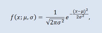
where parameter μ — is the mean (expectation) of a random variable and indicates the maximum coordinate of the distribution density curve, and σ² is the variance.

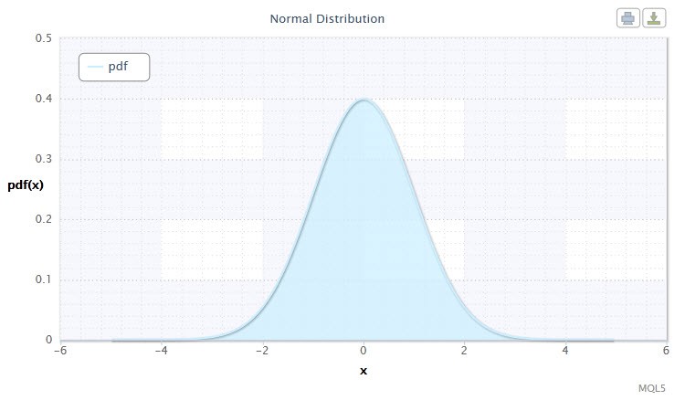
Figure 1. Normal distribution density Nor(0,1)

Its notation has the following format: X ~ Nor(μ, σ²), where:

X is a random variable selected from the normal distribution Nor;
μ is the mean parameter (-∞ ≤ μ ≤ +∞);
σ is the variance parameter (0<σ).

Valid range of the random variable X: -∞ ≤ X ≤ +∞.

The formulas used in this article may vary from those provided in other sources. Such difference is sometimes not mathematically crucial. In some instances it is conditional upon differences in parameterisation.

Normal distribution plays an important role in statistics as it reflects regularity arising as a result of interaction between a great number of random causes, none of which has a prevailing power. And although the normal distribution is a rare instance in financial markets, it is nevertheless important to compare it with empirical distributions in order to determine the extent and nature of their abnormality.

Let's define CNormaldist class for the normal distribution as follows:

//+------------------------------------------------------------------+
//|                Normal Distribution class definition              |
//+------------------------------------------------------------------+
class CNormaldist : CErf // Erf class inheritance
  {
public:
   double            mu, //mean parameter (μ)
   sig;                 //variance parameter (σ)
   //+------------------------------------------------------------------+
   //| CNormaldist class constructor                                    |
   //+------------------------------------------------------------------+
   void  CNormaldist()
     {
      mu=0.0;sig=1.0; //default parameters μ and σ
      if(sig<=0.) Alert("bad sig in Normal Distribution!");
     }
   //+------------------------------------------------------------------+
   //| Probability density function (pdf)                               |
   //+------------------------------------------------------------------+
   double pdf(double x)
     {
      return(0.398942280401432678/sig)*exp(-0.5*pow((x-mu)/sig,2));
     }
   //+------------------------------------------------------------------+
   //| Cumulative distribution function (cdf)                           |
   //+------------------------------------------------------------------+
   double cdf(double x)
     {
      return 0.5*erfc(-0.707106781186547524*(x-mu)/sig);
     }
   //+------------------------------------------------------------------+
   //| Inverse cumulative distribution function (invcdf)                |
   //| quantile function                                                |
   //+------------------------------------------------------------------+
   double invcdf(double p)
     {
      if(!(p>0. && p<1.))
         Alert("bad p in Normal Distribution!");
      return -1.41421356237309505*sig*inverfc(2.*p)+mu;
     }
   //+------------------------------------------------------------------+
   //| Reliability (survival) function (sf)                             |
   //+------------------------------------------------------------------+
   double sf(double x)
     {
      return 1-cdf(x);
     }
  };

//+------------------------------------------------------------------+

As you can notice, CNormaldist class derives from СErf base class which in its turn defines the error function class. It will be required upon calculation of some CNormaldist class methods. СErf class and auxiliary function erfcc look more or less like this:

//+------------------------------------------------------------------+
//|                Error Function class definition                   |
//+------------------------------------------------------------------+
class CErf
  {
public:
   int               ncof;    // coefficient array size
   double            cof[28]; // Chebyshev coefficient array
   //+------------------------------------------------------------------+
   //| CErf class constructor                                           |
   //+------------------------------------------------------------------+
   void CErf()
     {
      int Ncof=28;
      double Cof[28]=//Chebyshev coefficients
        {
         -1.3026537197817094,6.4196979235649026e-1,
         1.9476473204185836e-2,-9.561514786808631e-3,-9.46595344482036e-4,
         3.66839497852761e-4,4.2523324806907e-5,-2.0278578112534e-5,
         -1.624290004647e-6,1.303655835580e-6,1.5626441722e-8,-8.5238095915e-8,
         6.529054439e-9,5.059343495e-9,-9.91364156e-10,-2.27365122e-10,
         9.6467911e-11, 2.394038e-12,-6.886027e-12,8.94487e-13, 3.13092e-13,
         -1.12708e-13,3.81e-16,7.106e-15,-1.523e-15,-9.4e-17,1.21e-16,-2.8e-17
        };
      setCErf(Ncof,Cof);
     };
   //+------------------------------------------------------------------+
   //| Set-method for ncof                                              |
   //+------------------------------------------------------------------+
   void setCErf(int Ncof,double &Cof[])
     {
      ncof=Ncof;
      ArrayCopy(cof,Cof);
     };
   //+------------------------------------------------------------------+
   //| CErf class destructor                                            |
   //+------------------------------------------------------------------+
   void ~CErf(){};
   //+------------------------------------------------------------------+
   //| Error function                                                   |
   //+------------------------------------------------------------------+
   double erf(double x)
     {
      if(x>=0.0) return 1.0-erfccheb(x);
      else return erfccheb(-x)-1.0;
     }
   //+------------------------------------------------------------------+
   //| Complementary error function                                     |
   //+------------------------------------------------------------------+
   double erfc(double x)
     {
      if(x>=0.0) return erfccheb(x);
      else return 2.0-erfccheb(-x);
     }
   //+------------------------------------------------------------------+
   //| Chebyshev approximations for the error function                  |
   //+------------------------------------------------------------------+
   double erfccheb(double z)
     {
      int j;
      double t,ty,tmp,d=0.0,dd=0.0;
      if(z<0.) Alert("erfccheb requires nonnegative argument!");
      t=2.0/(2.0+z);
      ty=4.0*t-2.0;
      for(j=ncof-1;j>0;j--)
        {
         tmp=d;
         d=ty*d-dd+cof[j];
         dd=tmp;
        }
      return t*exp(-z*z+0.5*(cof[0]+ty*d)-dd);
     }
   //+------------------------------------------------------------------+
   //| Inverse complementary error function                             |
   //+------------------------------------------------------------------+
   double inverfc(double p)
     {
      double x,err,t,pp;
      if(p >= 2.0) return -100.0;
      if(p <= 0.0) return 100.0;
      pp=(p<1.0)? p : 2.0-p;
      t = sqrt(-2.*log(pp/2.0));
      x = -0.70711*((2.30753+t*0.27061)/(1.0+t*(0.99229+t*0.04481)) - t);
      for(int j=0;j<2;j++)
        {
         err=erfc(x)-pp;
         x+=err/(M_2_SQRTPI*exp(-pow(x,2))-x*err);
        }
      return(p<1.0? x : -x);
     }
   //+------------------------------------------------------------------+
   //| Inverse error function                                           |
   //+------------------------------------------------------------------+
   double inverf(double p)
     {return inverfc(1.0-p);}
  };
//+------------------------------------------------------------------+
double erfcc(const double x)
/* 
 complementary error function erfc(x) with
 a relative error of 1.2 * 10^(-7)               
*/
  {
   double t,z=fabs(x),ans;
   t=2./(2.0+z);
   ans=t*exp(-z*z-1.26551223+t*(1.00002368+t*(0.37409196+t*(0.09678418+
             t*(-0.18628806+t*(0.27886807+t*(-1.13520398+t*(1.48851587+
             t*(-0.82215223+t*0.17087277)))))))));
   return(x>=0.0 ? ans : 2.0-ans);
  }
//+------------------------------------------------------------------+

2.1.2 Log-Normal Distribution

Now let's have a look at the log-normal distribution.

Log-normal distribution in probability theory is a two-parameter family of absolutely continuous distributions. If a random variable is log-normally distributed, its logarithm has a normal distribution.

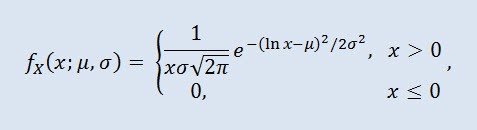
where μ is the location parameter (0<μ ), and σ is the scale parameter (0<σ).

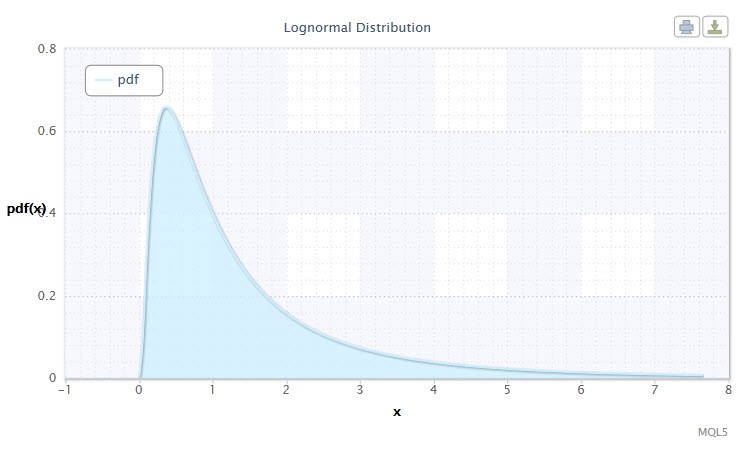
Figure 2. Log-normal distribution density Logn(0,1)

Its notation has the following format: X ~ Logn(μ, σ²), where:

X is a random variable selected from the log-normal distribution Logn;
μ is the location parameter (0<μ );
σ is the scale parameter (0<σ).

Valid range of the random variable X: 0 ≤ X ≤ +∞.

Let's create CLognormaldist сlass describing the log-normal distribution. It will appear as follows:

//+------------------------------------------------------------------+
//|                Lognormal Distribution class definition           |
//+------------------------------------------------------------------+
class CLognormaldist : CErf // Erf class inheritance
  {
public:
   double            mu, //location parameter (μ)
   sig;                 //scale parameter (σ)
   //+------------------------------------------------------------------+
   //| CLognormaldist class constructor                                 |
   //+------------------------------------------------------------------+
   void  CLognormaldist()
     {
      mu=0.0;sig=1.0; //default parameters μ and σ
      if(sig<=0.) Alert("bad sig in Lognormal Distribution!");
     }
   //+------------------------------------------------------------------+
   //| Probability density function (pdf)                               |
   //+------------------------------------------------------------------+
   double pdf(double x)
     {
      if(x<0.) Alert("bad x in Lognormal Distribution!");
      if(x==0.) return 0.;
      return(0.398942280401432678/(sig*x))*exp(-0.5*pow((log(x)-mu)/sig,2));
     }
   //+------------------------------------------------------------------+
   //| Cumulative distribution function (cdf)                           |
   //+------------------------------------------------------------------+
   double cdf(double x)
     {
      if(x<0.) Alert("bad x in Lognormal Distribution!");
      if(x==0.) return 0.;
      return 0.5*erfc(-0.707106781186547524*(log(x)-mu)/sig);
     }
   //+------------------------------------------------------------------+
   //| Inverse cumulative distribution function (invcdf)(quantile)      |
   //+------------------------------------------------------------------+
   double invcdf(double p)
     {
      if(!(p>0. && p<1.))
         Alert("bad p in Lognormal Distribution!");
      return exp(-1.41421356237309505*sig*inverfc(2.*p)+mu);
     }
   //+------------------------------------------------------------------+
   //| Reliability (survival) function (sf)                             |
   //+------------------------------------------------------------------+
   double sf(double x)
     {
      return 1-cdf(x);
     }
  };
//+------------------------------------------------------------------+

As can be seen, the log-normal distribution is not much different from the normal distribution. The difference being that the parameter x is replaced by the parameter log(x).

2.1.3 Cauchy Distribution

Cauchy distribution in probability theory (in physics also called Lorentz distribution or Breit-Wigner distribution) is a class of absolutely continuous distributions. A Cauchy distributed random variable is a common example of a variable that has no expectation and no variance. The density takes the following form:

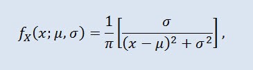
where μ is the location parameter (-∞ ≤ μ ≤ +∞ ), and σ is the scale parameter (0<σ).

The notation of the Cauchy distribution has the following format: X ~ Cau(μ, σ), where:

X is a random variable selected from the Cauchy distribution Cau;
μ is the location parameter (-∞ ≤ μ ≤ +∞ );
σ is the scale parameter (0<σ).

Valid range of the random variable X: -∞ ≤ X ≤ +∞.

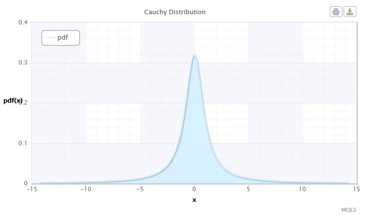
Figure 3. Cauchy distribution density Cau(0,1)

Created with the help of CCauchydist class, in MQL5 format it looks as follows:

//+------------------------------------------------------------------+
//|                Cauchy Distribution class definition              |
//+------------------------------------------------------------------+
class CCauchydist //
  {
public:
   double            mu,//location parameter (μ)
   sig;                 //scale parameter (σ)
   //+------------------------------------------------------------------+
   //| CCauchydist class constructor                                    |
   //+------------------------------------------------------------------+
   void  CCauchydist() 
     {
      mu=0.0;sig=1.0; //default parameters μ and σ
      if(sig<=0.) Alert("bad sig in Cauchy Distribution!");
     }
   //+------------------------------------------------------------------+
   //| Probability density function (pdf)                               |
   //+------------------------------------------------------------------+
   double pdf(double x)
     {
      return 0.318309886183790671/(sig*(1.+pow((x-mu)/sig,2)));
     }
   //+------------------------------------------------------------------+
   //| Cumulative distribution function (cdf)                           |
   //+------------------------------------------------------------------+
   double cdf(double x)
     {
      return 0.5+0.318309886183790671*atan2(x-mu,sig); //todo      
     }
   //+------------------------------------------------------------------+
   //| Inverse cumulative distribution function (invcdf) (quantile func)|
   //+------------------------------------------------------------------+
   double invcdf(double p)
     {
      if(!(p>0. && p<1.))
         Alert("bad p in Cauchy Distribution!");
      return mu+sig*tan(M_PI*(p-0.5));
     }
   //+------------------------------------------------------------------+
   //| Reliability (survival) function (sf)                             |
   //+------------------------------------------------------------------+
   double sf(double x)
     {
      return 1-cdf(x);
     }
  };
//+------------------------------------------------------------------+

It should be noted here that atan2() function is utilized, which returns the principal value of arc tangent in radians:

double atan2(double y,double x)
/*
 Returns the principal value of the arc tangent of y/x,
 expressed in radians. To compute the value, the function 
 uses the sign of both arguments to determine the quadrant.
 y - double value representing an y-coordinate.
 x - double value representing an x-coordinate. 
*/
  {
   double a;
   if(fabs(x)>fabs(y))
      a=atan(y/x);
   else
     {
      a=atan(x/y); // pi/4 <= a <= pi/4
      if(a<0.)
         a=-1.*M_PI_2-a; //a is negative, so we're adding
      else
         a=M_PI_2-a;
     }
   if(x<0.)
     {
      if(y<0.)
         a=a-M_PI;
      else
         a=a+M_PI;
     }
   return a;
  }

2.1.4 Hyperbolic Secant Distribution

Hyperbolic secant distribution will be of interest to those who deal with financial rank analysis.

In probability theory and statistics, the hyperbolic secant distribution is a continuous probability distribution whose probability density function and characteristic function are proportional to the hyperbolic secant function. The density is given by the formula:

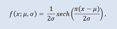
where μ is the location parameter (-∞ ≤ μ ≤ +∞ ), and σ is the scale parameter (0<σ).

Figure 4. Hyperbolic secant distribution density HS(0,1)

Its notation has the following format: X ~ HS(μ, σ), where:

X is a random variable;
μ is the location parameter (-∞ ≤ μ ≤ +∞ );
σ is the scale parameter (0<σ).

Valid range of the random variable X: -∞ ≤ X ≤ +∞.

Let's describe it utilizing CHypersecdist class as follows:

//+------------------------------------------------------------------+
//|        Hyperbolic Secant Distribution class definition           |
//+------------------------------------------------------------------+
class CHypersecdist //
  {
public:
   double            mu,// location parameter (μ)
   sig;                 //scale parameter (σ)
   //+------------------------------------------------------------------+
   //| CHypersecdist class constructor                                 |
   //+------------------------------------------------------------------+
   void  CHypersecdist()
     {
      mu=0.0;sig=1.0; //default parameters μ and σ
      if(sig<=0.) Alert("bad sig in Hyperbolic Secant Distribution!");
     }
   //+------------------------------------------------------------------+
   //| Probability density function (pdf)                               |
   //+------------------------------------------------------------------+
   double pdf(double x)
     {
      return sech((M_PI*(x-mu))/(2*sig))/2*sig;
     }
   //+------------------------------------------------------------------+
   //| Cumulative distribution function (cdf)                           |
   //+------------------------------------------------------------------+
   double cdf(double x)
     {
      return 2/M_PI*atan(exp((M_PI*(x-mu)/(2*sig))));
     }
   //+------------------------------------------------------------------+
   //| Inverse cumulative distribution function (invcdf) (quantile func)|
   //+------------------------------------------------------------------+
   double invcdf(double p)
     {
      if(!(p>0. && p<1.))
         Alert("bad p in Hyperbolic Secant Distribution!");
      return(mu+(2.0*sig/M_PI*log(tan(M_PI/2.0*p))));
     }
   //+------------------------------------------------------------------+
   //| Reliability (survival) function (sf)                             |
   //+------------------------------------------------------------------+
   double sf(double x)
     {
      return 1-cdf(x);
     }
  };
//+------------------------------------------------------------------+

It is not difficult to see that this distribution has got its name from the hyperbolic secant function whose probability density function is proportional to the hyperbolic secant function.

Hyperbolic secant function sech is as follows:

//+------------------------------------------------------------------+
//|              Hyperbolic Secant Function                          |
//+------------------------------------------------------------------+
double sech(double x)
// Hyperbolic Secant Function
  {
   return 2/(pow(M_E,x)+pow(M_E,-x));
  }

2.1.5 Student's t-Distribution

Student's t-distribution is an important distribution in statistics.

In probability theory, Student's t-distribution is most often a one-parameter family of absolutely continuous distributions. However it can also be considered a three-parameter distribution that is given by the distribution density function:

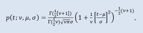
where Г is Euler's Gamma function, ν is the shape parameter (ν>0), μ is the location parameter (-∞ ≤ μ ≤ +∞ ), σ is the scale parameter (0<σ).

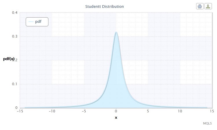
Figure 5. Student's t-distribution density Stt(1,0,1)

Its notation has the following format: t ~ Stt(ν,μ,σ), where:

t is a random variable selected from the Student's t-distribution Stt;
ν is the shape parameter (ν>0)
μ is the location parameter (-∞ ≤ μ ≤ +∞ );
σ is the scale parameter (0<σ).

Valid range of the random variable X: -∞ ≤ X ≤ +∞.

Often, especially in hypothesis testing a standard t-distribution is used with μ=0 and σ=1. Thus, it turns into a one-parameter distribution with parameter ν.

This distribution is often used in estimating the expectation, projected values and other characteristics by means of confidence intervals, when testing expectation value hypotheses, regression relationship coefficients, homogeneity hypotheses, etc.

Let's describe the distribution through CStudenttdist class:

//+------------------------------------------------------------------+
//|                Student's t-distribution class definition         |
//+------------------------------------------------------------------+
class CStudenttdist : CBeta // CBeta class inheritance
  {
public:
   int               nu;     // shape parameter (ν)
   double            mu,     // location parameter (μ)
   sig,                     // scale parameter (σ)
   np,                      // 1/2*(ν+1)
   fac;                     // Г(1/2*(ν+1))-Г(1/2*ν)
   //+------------------------------------------------------------------+
   //| CStudenttdist class constructor                                  |
   //+------------------------------------------------------------------+
   void  CStudenttdist()
     {
      int Nu=1;double Mu=0.0,Sig=1.0; //default parameters ν, μ and σ
      setCStudenttdist(Nu,Mu,Sig);
     }
   void setCStudenttdist(int Nu,double Mu,double Sig)
     {
      nu=Nu;
      mu=Mu;
      sig=Sig;
      if(sig<=0. || nu<=0.) Alert("bad sig,nu in Student-t Distribution!");
      np=0.5*(nu+1.);
      fac=gammln(np)-gammln(0.5*nu);
     }
   //+------------------------------------------------------------------+
   //| Probability density function (pdf)                               |
   //+------------------------------------------------------------------+
   double pdf(double x)
     {
      return exp(-np*log(1.+pow((x-mu)/sig,2.)/nu)+fac)/(sqrt(M_PI*nu)*sig);
     }
   //+------------------------------------------------------------------+
   //| Cumulative distribution function (cdf)                           |
   //+------------------------------------------------------------------+
   double cdf(double t)
     {
      double p=0.5*betai(0.5*nu,0.5,nu/(nu+pow((t-mu)/sig,2)));
      if(t>=mu) return 1.-p;
      else return p;
     }
   //+------------------------------------------------------------------+
   //| Inverse cumulative distribution function (invcdf) (quantile func)|
   //+------------------------------------------------------------------+
   double invcdf(double p)
     {
      if(p<=0. || p>=1.) Alert("bad p in Student-t Distribution!");
      double x=invbetai(2.*fmin(p,1.-p),0.5*nu,0.5);
      x=sig*sqrt(nu*(1.-x)/x);
      return(p>=0.5? mu+x : mu-x);
     }
   //+------------------------------------------------------------------+
   //| Reliability (survival) function (sf)                             |
   //+------------------------------------------------------------------+
   double sf(double x)
     {
      return 1-cdf(x);
     }
   //+------------------------------------------------------------------+
   //| Two-tailed cumulative distribution function (aa) A(t|ν)          |
   //+------------------------------------------------------------------+
   double aa(double t)
     {
      if(t < 0.) Alert("bad t in Student-t Distribution!");
      return 1.-betai(0.5*nu,0.5,nu/(nu+pow(t,2.)));
     }
   //+------------------------------------------------------------------+
   //| Inverse two-tailed cumulative distribution function (invaa)      |
   //| p=A(t|ν)                                                         |
   //+------------------------------------------------------------------+
   double invaa(double p)
     {
      if(!(p>=0. && p<1.)) Alert("bad p in Student-t Distribution!");
      double x=invbetai(1.-p,0.5*nu,0.5);
      return sqrt(nu*(1.-x)/x);
     }
  };
//+------------------------------------------------------------------+

The CStudenttdist class listing shows that CBeta is a base class which describes the incomplete beta function.

CBeta class appears as follows:

//+------------------------------------------------------------------+
//|            Incomplete Beta Function class definition             |
//+------------------------------------------------------------------+
class CBeta : public CGauleg18
  {
private:
   int               Switch;                     //when to use the quadrature method
   double            Eps,Fpmin;
public:
   //+------------------------------------------------------------------+
   //| CBeta class constructor                                          |
   //+------------------------------------------------------------------+
   void CBeta()
     {
      int swi=3000;
      setCBeta(swi,EPS,FPMIN);
     };
   //+------------------------------------------------------------------+
   //| CBeta class set-method                                           |
   //+------------------------------------------------------------------+
   void setCBeta(int swi,double eps,double fpmin)
     {
      Switch=swi;
      Eps=eps;
      Fpmin=fpmin;
     };
   double            betai(const double a,const double b,const double x); //incomplete beta function Ix(a,b)
   double            betacf(const double a,const double b,const double x);//continued fraction for incomplete beta function
   double            betaiapprox(double a,double b,double x); //Incomplete beta by quadrature
   double            invbetai(double p,double a,double b);    //Inverse of incomplete beta function
  };

This class also has a base class CGauleg18 which provides coefficients for such numerical integration method as Gauss-Legendre quadrature.

2.1.6 Logistic Distribution

I propose to consider the logistic distribution the next in our study.

In probability theory and statistics, the logistic distribution is a continuous probability distribution. Its cumulative distribution function is the logistic function. It resembles the normal distribution in shape but has heavier tails. Distribution density:

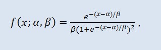
where α is the location parameter (-∞ ≤ α ≤ +∞ ), β is the scale parameter (0<β).

Figure 6. Logistic distribution density Logi(0,1)

Its notation has the following format: X ~ Logi(α,β), where:

X is a random variable;
α is the location parameter (-∞ ≤ α ≤ +∞ );
β is the scale parameter (0<β).

Valid range of the random variable X: -∞ ≤ X ≤ +∞.

CLogisticdist class is the implementation of the above described distribution:

//+------------------------------------------------------------------+
//|                Logistic Distribution class definition            |
//+------------------------------------------------------------------+
class CLogisticdist
  {
public:
   double            alph,//location parameter (α)
   bet;                   //scale parameter (β)
   //+------------------------------------------------------------------+
   //| CLogisticdist class constructor                                  |
   //+------------------------------------------------------------------+
   void  CLogisticdist() 
     {
      alph=0.0;bet=1.0; //default parameters μ and σ
      if(bet<=0.) Alert("bad bet in Logistic Distribution!");
     }
   //+------------------------------------------------------------------+
   //| Probability density function (pdf)                               |
   //+------------------------------------------------------------------+
   double pdf(double x)
     {
      return exp(-(x-alph)/bet)/(bet*pow(1.+exp(-(x-alph)/bet),2));
     }
   //+------------------------------------------------------------------+
   //| Cumulative distribution function (cdf)                           |
   //+------------------------------------------------------------------+
   double cdf(double x)
     {
      double et=exp(-1.*fabs(1.81379936423421785*(x-alph)/bet));
      if(x>=alph) return 1./(1.+et);
      else return et/(1.+et);
     }
   //+------------------------------------------------------------------+
   //| Inverse cumulative distribution function (invcdf) (quantile func)|
   //+------------------------------------------------------------------+
   double invcdf(double p)
     {
      if(p<=0. || p>=1.) Alert("bad p in Logistic Distribution!");
      return alph+0.551328895421792049*bet*log(p/(1.-p));
     }
   //+------------------------------------------------------------------+
   //| Reliability (survival) function (sf)                             |
   //+------------------------------------------------------------------+
   double sf(double x)
     {
      return 1-cdf(x);
     }
  };
//+------------------------------------------------------------------+

2.1.7 Exponential Distribution

Let's also have a look at the exponential distribution of a random variable.

A random variable X has the exponential distribution with parameter λ > 0, if its density is given by:

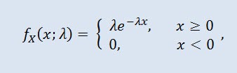
where λ is the scale parameter (λ>0).

Figure 7. Exponential distribution density Exp(1)

Its notation has the following format: X ~ Exp(λ), where:

X is a random variable;
λ is the scale parameter (λ>0).

Valid range of the random variable X: 0 ≤ X ≤ +∞.

This distribution is remarkable for the fact that it describes a sequence of events taking place one by one at certain times. Thus, using this distribution a trader can analyze a series of loss deals and others.

In MQL5 code, the distribution is described through CExpondist class:

//+------------------------------------------------------------------+
//|                Exponential Distribution class definition         |
//+------------------------------------------------------------------+
class CExpondist
  {
public:
   double            lambda;   //scale parameter (λ)
   //+------------------------------------------------------------------+
   //| CExpondist class constructor                                     |
   //+------------------------------------------------------------------+
   void  CExpondist()
     {
      lambda=1.0;              //default parameter λ
      if(lambda<=0.) Alert("bad lambda in Exponential Distribution!");
     }
   //+------------------------------------------------------------------+
   //| Probability density function (pdf)                               |
   //+------------------------------------------------------------------+
   double pdf(double x)
     {
      if(x<0.) Alert("bad x in Exponential Distribution!");
      return lambda*exp(-lambda*x);
     }
   //+------------------------------------------------------------------+
   //| Cumulative distribution function (cdf)                           |
   //+------------------------------------------------------------------+
   double cdf(double x)
     {
      if(x < 0.) Alert("bad x in Exponential Distribution!");
      return 1.-exp(-lambda*x);
     }
   //+------------------------------------------------------------------+
   //| Inverse cumulative distribution function (invcdf) (quantile func)|
   //+------------------------------------------------------------------+
   double invcdf(double p)
     {
      if(p<0. || p>=1.) Alert("bad p in Exponential Distribution!");
      return -log(1.-p)/lambda;
     }
   //+------------------------------------------------------------------+
   //| Reliability (survival) function (sf)                             |
   //+------------------------------------------------------------------+
   double sf(double x)
     {
      return 1-cdf(x);
     }
  };
//+------------------------------------------------------------------+

2.1.8 Gamma Distribution

I've chosen the gamma distribution as the next type of the random variable continuous distribution.

In probability theory, the gamma distribution is a two-parameter family of absolutely continuous probability distributions. If parameter α is an integer, such gamma distribution is also called the Erlang distribution. The density takes the following form:

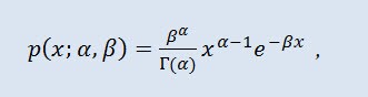
where Г is Euler's Gamma function, α is the shape parameter (0<α), β is the scale parameter (0<β).

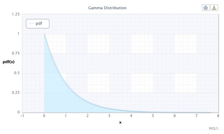
Figure 8. Gamma distribution density Gam(1,1).

Its notation has the following format: X ~ Gam(α,β), where:

X is a random variable;
α is the shape parameter (0<α);
β is the scale parameter (0<β).

Valid range of the random variable X: 0 ≤ X ≤ +∞.

In CGammadist class-defined variant it looks as follows:

//+------------------------------------------------------------------+
//|                Gamma Distribution class definition               |
//+------------------------------------------------------------------+
class CGammadist : CGamma // CGamma class inheritance
  {
public:
   double            alph,//continuous shape parameter (α>0)
   bet,                   //continuous scale parameter  (β>0)
   fac;                   //factor
   //+------------------------------------------------------------------+
   //| CGammaldist class constructor                                    |
   //+------------------------------------------------------------------+
   void  CGammadist()
     {
      setCGammadist();
     }
   void setCGammadist(double Alph=1.0,double Bet=1.0)//default parameters α and β
     {
      alph=Alph; bet=Bet;
      if(alph<=0. || bet<=0.) Alert("bad alph,bet in Gamma Distribution!");
      fac=alph*log(bet)-gammln(alph);
     }
   //+------------------------------------------------------------------+
   //| Probability density function (pdf)                               |
   //+------------------------------------------------------------------+
   double pdf(double x)
     {
      if(x<=0.) Alert("bad x in Gamma Distribution!");
      return exp(-bet*x+(alph-1.)*log(x)+fac);
     }
   //+------------------------------------------------------------------+
   //| Cumulative distribution function (cdf)                           |
   //+------------------------------------------------------------------+
   double cdf(double x)
     {
      if(x<0.) Alert("bad x in Gamma Distribution!");
      return gammp(alph,bet*x);
     }
   //+------------------------------------------------------------------+
   //| Inverse cumulative distribution function (invcdf) (quantile func)|
   //+------------------------------------------------------------------+
   double invcdf(double p)
     {
      if(p<0. || p>=1.) Alert("bad p in Gamma Distribution!");
      return invgammp(p,alph)/bet;
     }
   //+------------------------------------------------------------------+
   //| Reliability (survival) function (sf)                             |
   //+------------------------------------------------------------------+
   double sf(double x)
     {
      return 1-cdf(x);
     }
  };
//+------------------------------------------------------------------+

Gamma distribution class derives from CGamma class that describes the incomplete gamma function.

CGamma class is defined as follows:

//+------------------------------------------------------------------+
//|            Incomplete Gamma Function class definition            |
//+------------------------------------------------------------------+
class CGamma : public CGauleg18
  {
private:
   int               ASWITCH;
   double            Eps,
   Fpmin,
   gln;
public:
   //+------------------------------------------------------------------+
   //| CGamma class constructor                                         |
   //+------------------------------------------------------------------+
   void CGamma()
     {
      int aswi=100;
      setCGamma(aswi,EPS,FPMIN);
     };
   void setCGamma(int aswi,double eps,double fpmin) //CGamma set-method
     {
      ASWITCH=aswi;
      Eps=eps;
      Fpmin=fpmin;
     };
   double            gammp(const double a,const double x); //incomplete gamma function
   double            gammq(const double a,const double x); //incomplete gamma function Q(a,x)
   void              gser(double &gamser,double a,double x,double &gln); //incomplete gamma function P(a,x)
   double            gcf(const double a,const double x); //incomplete gamma function Q(a,x)
   double            gammpapprox(double a,double x,int psig); //incomplete gamma by quadrature
   double            invgammp(double p,double a); //inverse of incomplete gamma function
  };
//+------------------------------------------------------------------+

Both CGamma class and CBeta class have CGauleg18 as a base class.

2.1.9 Beta Distribution

Well, let us now review the beta distribution.

In probability theory and statistics, the beta distribution is a two-parameter family of absolutely continuous distributions. It is used to describe the random variables whose values are defined on a finite interval. The density is defined as follows:

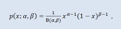
where B is the beta function, α is the 1st shape parameter (0<α), β is the 2nd shape parameter (0<β).

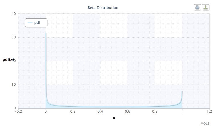
Figure 9. Beta distribution density Beta(0.5,0.5)

Its notation has the following format: X ~ Beta(α,β), where:

X is a random variable;
α is the 1st shape parameter (0<α);
β is the 2nd shape parameter (0<β).

Valid range of the random variable X: 0 ≤ X ≤ 1.

CBetadist class describes this distribution in the following way:

//+------------------------------------------------------------------+
//|                Beta Distribution class definition                |
//+------------------------------------------------------------------+
class CBetadist : CBeta // CBeta class inheritance
  {
public:
   double            alph,//continuous shape parameter (α>0)
   bet,                   //continuous shape parameter (β>0)
   fac;                   //factor
   //+------------------------------------------------------------------+
   //| CBetadist class constructor                                      |
   //+------------------------------------------------------------------+
   void  CBetadist()
     {
      setCBetadist();
     }
   void setCBetadist(double Alph=0.5,double Bet=0.5)//default parameters α and β
     {
      alph=Alph; bet=Bet;
      if(alph<=0. || bet<=0.) Alert("bad alph,bet in Beta Distribution!");
      fac=gammln(alph+bet)-gammln(alph)-gammln(bet);
     }
   //+------------------------------------------------------------------+
   //| Probability density function (pdf)                               |
   //+------------------------------------------------------------------+
   double pdf(double x)
     {
      if(x<=0. || x>=1.) Alert("bad x in Beta Distribution!");
      return exp((alph-1.)*log(x)+(bet-1.)*log(1.-x)+fac);
     }
   //+------------------------------------------------------------------+
   //| Cumulative distribution function (cdf)                           |
   //+------------------------------------------------------------------+
   double cdf(double x)
     {
      if(x<0. || x>1.) Alert("bad x in Beta Distribution");
      return betai(alph,bet,x);
     }
   //+------------------------------------------------------------------+
   //| Inverse cumulative distribution function (invcdf) (quantile func)|
   //+------------------------------------------------------------------+
   double invcdf(double p)
     {
      if(p<0. || p>1.) Alert("bad p in Beta Distribution!");
      return invbetai(p,alph,bet);
     }
   //+------------------------------------------------------------------+
   //| Reliability (survival) function (sf)                             |
   //+------------------------------------------------------------------+
   double sf(double x)
     {
      return 1-cdf(x);
     }
  };
//+------------------------------------------------------------------+

2.1.10 Laplace Distribution

Another remarkable continuous distribution is the Laplace distribution (double exponential distribution).

The Laplace distribution (double exponential distribution) in probability theory is a continuous distribution of a random variable whereby the probability density is:

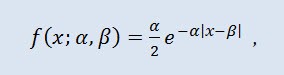
where α is the location parameter (-∞ ≤ α ≤ +∞ ), β is the scale parameter (0<β).

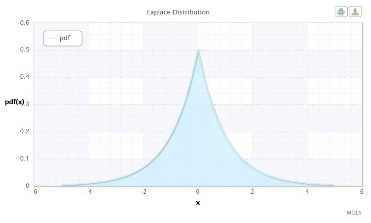
Figure 10. Laplace distribution density Lap(0,1)

Its notation has the following format: X ~ Lap(α,β), where:

X is a random variable;
α is the location parameter (-∞ ≤ α ≤ +∞ );
β is the scale parameter (0<β).

Valid range of the random variable X: -∞ ≤ X ≤ +∞.

CLaplacedist class for purposes of this distribution is defined as follows:

//+------------------------------------------------------------------+
//|                 Laplace Distribution class definition            |
//+------------------------------------------------------------------+
class CLaplacedist
  {
public:
   double            alph;   //location parameter (α)
   double            bet;    //scale parameter (β)
   //+------------------------------------------------------------------+
   //| CLaplacedist class constructor                                   |
   //+------------------------------------------------------------------+
   void  CLaplacedist()
     {
      alph=.0;               //default parameter α
      bet=1.;                //default parameter β
      if(bet<=0.) Alert("bad bet in Laplace Distribution!");
     }
   //+------------------------------------------------------------------+
   //| Probability density function (pdf)                               |
   //+------------------------------------------------------------------+
   double pdf(double x)
     {
      return exp(-fabs((x-alph)/bet))/2*bet;
     }
   //+------------------------------------------------------------------+
   //| Cumulative distribution function (cdf)                           |
   //+------------------------------------------------------------------+
   double cdf(double x)
     {
      double temp;
      if(x<0)
         temp=0.5*exp(-fabs((x-alph)/bet));
      else
         temp=1.-0.5*exp(-fabs((x-alph)/bet));
      return temp;
     }
   //+------------------------------------------------------------------+
   //| Inverse cumulative distribution function (invcdf) (quantile func)|
   //+------------------------------------------------------------------+
   double invcdf(double p)
     {
      double temp;
      if(p<0. || p>=1.) Alert("bad p in Laplace Distribution!");
      if(p<0.5)
         temp=bet*log(2*p)+alph;
      else
         temp=-1.*(bet*log(2*(1.-p))+alph);
      return temp;
     }
   //+------------------------------------------------------------------+
   //| Reliability (survival) function (sf)                             |
   //+------------------------------------------------------------------+
   double sf(double x)
     {
      return 1-cdf(x);
     }
  };
//+------------------------------------------------------------------+

So, utilizing MQL5 code we have created 10 classes for the ten continuous distributions. Apart from those, some more classes were created that were, so to say, complementary since there was a need in specific functions and methods (e.g. CBeta and CGamma).

Now let us proceed to the discrete distributions and create a few classes for this distribution category.

2.2.1 Binomial Distribution

Let's start with the binomial distribution.

In probability theory, the binomial distribution is a distribution of the number of successes in a sequence of independent random experiments where the success probability in every one of them is equal. The probability density is given by the following formula:

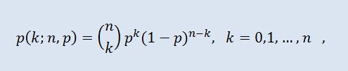
where (n k) is the binomial coefficient, n is the number of trials (0 ≤ n), p is the success probability (0 ≤ p ≤1).

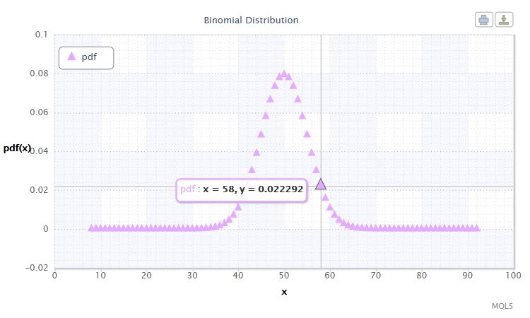
Figure 11. Binomial distribution density Bin(100,0.5).

Its notation has the following format: k ~ Bin(n,p), where:

k is a random variable;
n is the number of trials (0 ≤ n);
p is the success probability (0 ≤ p ≤1).

Valid range of the random variable X: 0 or 1.

Does the range of possible values of the random variable X suggest anything to you? Indeed, this distribution can help us analyze the aggregate of win (1) and loss (0) deals in the trading system.

Let's create СBinomialdist class as follows:

//+------------------------------------------------------------------+
//|               Binomial Distribution class definition             |
//+------------------------------------------------------------------+
class CBinomialdist : CBeta // CBeta class inheritance
  {
public:
   int               n;      //number of trials
   double            pe,     //success probability
   fac;                      //factor
   //+------------------------------------------------------------------+
   //| CBinomialdist class constructor                                  |
   //+------------------------------------------------------------------+
   void              CBinomialdist()
     {
      setCBinomialdist();
     }
   void setCBinomialdist(int N=100,double Pe=0.5)//default parameters n and pe
     {
      n=N; pe=Pe;
      if(n<=0 || pe<=0. || pe>=1.) Alert("bad args in Binomial Distribution!");
      fac=gammln(n+1.);
     }
   //+------------------------------------------------------------------+
   //| Probability density function (pdf)                               |
   //+------------------------------------------------------------------+
   double pdf(int k)
     {
      if(k<0) Alert("bad k in Binomial Distribution!");
      if(k>n) return 0.;
      return exp(k*log(pe)+(n-k)*log(1.-pe)+fac-gammln(k+1.)-gammln(n-k+1.));
     }
   //+------------------------------------------------------------------+
   //| Cumulative distribution function (cdf)                           |
   //+------------------------------------------------------------------+
   double cdf(int k)
     {
      if(k<0) Alert("bad k in Binomial Distribution!");
      if(k==0) return 0.;
      if(k>n) return 1.;
      return 1.-betai((double)k,n-k+1.,pe);
     }
   //+------------------------------------------------------------------+
   //| Inverse cumulative distribution function (invcdf) (quantile func)|
   //+------------------------------------------------------------------+
   int invcdf(double p)
     {
      int k,kl,ku,inc=1;
      if(p<=0. || p>=1.) Alert("bad p in Binomial Distribution!");
      k=fmax(0,fmin(n,(int)(n*pe)));
      if(p<cdf(k))
        {
         do
           {
            k=fmax(k-inc,0);
            inc*=2;
           }
         while(p<cdf(k));
         kl=k; ku=k+inc/2;
           } else {
         do
           {
            k=fmin(k+inc,n+1);
            inc*=2;
           }
         while(p>cdf(k));
         ku=k; kl=k-inc/2;
        }
      while(ku-kl>1)
        {
         k=(kl+ku)/2;
         if(p<cdf(k)) ku=k;
         else kl=k;
        }
      return kl;
     }
   //+------------------------------------------------------------------+
   //| Reliability (survival) function (sf)                             |
   //+------------------------------------------------------------------+
   double sf(int k)
     {
      return 1.-cdf(k);
     }
  };
//+------------------------------------------------------------------+

2.2.2 Poisson Distribution

The next distribution under review is the Poisson distribution.

The Poisson distribution models a random variable represented by a number of events occurring over a fixed period of time, provided that these events occur with a fixed average intensity and independently of one another. The density takes the following form:

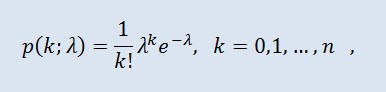
where k! is the factorial, λ is the location parameter (0 < λ).

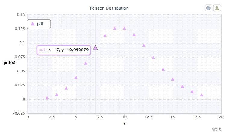
Figure 12. Poisson distribution density Pois(10).

Its notation has the following format: k ~ Pois(λ), where:

k is a random variable;
λ is the location parameter (0 < λ).

Valid range of the random variable X: 0 ≤ X ≤ +∞.

The Poisson distribution describes the "law of rare events" which is important when estimating the degree of risk.

CPoissondist class will serve the purposes of this distribution:

//+------------------------------------------------------------------+
//|               Poisson Distribution class definition              |
//+------------------------------------------------------------------+
class CPoissondist : CGamma // CGamma class inheritance
  {
public:
   double            lambda;   //location parameter (λ)
   //+------------------------------------------------------------------+
   //| CPoissondist class constructor                                   |
   //+------------------------------------------------------------------+
   void CPoissondist()
     {
      lambda=15.;
      if(lambda<=0.) Alert("bad lambda in Poisson Distribution!");
     }
   //+------------------------------------------------------------------+
   //| Probability density function (pdf)                               |
   //+------------------------------------------------------------------+
   double pdf(int n)
     {
      if(n<0) Alert("bad n in Poisson Distribution!");
      return exp(-lambda+n*log(lambda)-gammln(n+1.));
     }
   //+------------------------------------------------------------------+
   //| Cumulative distribution function (cdf)                           |
   //+------------------------------------------------------------------+
   double cdf(int n)
     {
      if(n<0) Alert("bad n in Poisson Distribution!");
      if(n==0) return 0.;
      return gammq((double)n,lambda);
     }
   //+------------------------------------------------------------------+
   //| Inverse cumulative distribution function (invcdf) (quantile func)|
   //+------------------------------------------------------------------+
   int invcdf(double p)
     {
      int n,nl,nu,inc=1;
      if(p<=0. || p>=1.) Alert("bad p in Poisson Distribution!");
      if(p<exp(-lambda)) return 0;
      n=(int)fmax(sqrt(lambda),5.);
      if(p<cdf(n))
        {
         do
           {
            n=fmax(n-inc,0);
            inc*=2;
           }
         while(p<cdf(n));
         nl=n; nu=n+inc/2;
           } else {
         do
           {
            n+=inc;
            inc*=2;
           }
         while(p>cdf(n));
         nu=n; nl=n-inc/2;
        }
      while(nu-nl>1)
        {
         n=(nl+nu)/2;
         if(p<cdf(n)) nu=n;
         else nl=n;
        }
      return nl;
     }
   //+------------------------------------------------------------------+
   //| Reliability (survival) function (sf)                             |
   //+------------------------------------------------------------------+
   double sf(int n)
     {
      return 1.-cdf(n);
     }
  };
//+=====================================================================+

It is obviously impossible to consider all statistical distributions within one article and probably not even necessary. The user, if so desired, may expand the distribution gallery set out above. Created distributions can be found in Distribution_class.mqh file.

3. Creating Distribution Graphs

Now I suggest we should see how the classes we created for the distributions can be used in our future work.

At this point, again utilizing OOP, I have created CDistributionFigure class that processes user-defined parameter distributions and displays them on the screen by means described in article "Charts and Diagrams in HTML".

//+------------------------------------------------------------------+
//|           Distribution Figure class definition                   |
//+------------------------------------------------------------------+
class CDistributionFigure
  {
private:
   Dist_type         type;  //distribution type
   Dist_mode         mode;  //distribution mode
   double            x;     //step start
   double            x11;   //left side limit
   double            x12;   //right side limit
   int               d;     //number of points
   double            st;    //step

public:
   double            xAr[]; //array of random variables
   double            p1[];  //array of probabilities
   void              CDistributionFigure();  //constructor 
   void              setDistribution(Dist_type Type,Dist_mode Mode,double X11,double X12,double St); //set-method
   void              calculateDistribution(double nn,double mm,double ss); //distribution parameter calculation
   void              filesave(); //saving distribution parameters
  };
//+------------------------------------------------------------------+

Omitting implementation. Note that this class has such data members as type and mode relating to Dist_type and Dist_mode correspondingly. These types are enumerations of the distributions under study and their types.

So, let's try to finally create a graph of some distribution.

I wrote continuousDistribution.mq5 script for continuous distributions, its key lines being as follows:

//+------------------------------------------------------------------+
//|                     Input variables                              |
//+------------------------------------------------------------------+

input Dist_type dist;  //Distribution Type
input Dist_mode distM; //Distribution Mode
input int nn=1;        //Nu
input double mm=0.,    //Mu
            ss=1.;    //Sigma
//+------------------------------------------------------------------+
//| Script program start function                                    |
//+------------------------------------------------------------------+
void OnStart()
  {
//(Normal #0,Lognormal #1,Cauchy #2,Hypersec #3,Studentt #4,Logistic #5,Exponential #6,Gamma #7,Beta #8 , Laplace #9)
   double Xx1,      //left side limit
          Xx2,     //right side limit          
          st=0.05; //step
   if(dist==0) //Normal
     {
      Xx1=mm-5.0*ss/1.25;
      Xx2=mm+5.0*ss/1.25;
     }
   if(dist==2 || dist==4 || dist==5) //Cauchy,Studentt,Logistic
     {
      Xx1=mm-5.0*ss/0.35;
      Xx2=mm+5.0*ss/0.35;
     }
   else if(dist==1 || dist==6 || dist==7) //Lognormal,Exponential,Gamma
     {
      Xx1=0.001;
      Xx2=7.75;
     }
   else if(dist==8) //Beta
     {
      Xx1=0.0001;
      Xx2=0.9999;
      st=0.001;
     }
   else 
     {
      Xx1=mm-5.0*ss;
      Xx2=mm+5.0*ss;
     }
//---
   CDistributionFigure F;        //creation of the CDistributionFigure class instance 
   F.setDistribution(dist,distM,Xx1,Xx2,st);
   F.calculateDistribution(nn,mm,ss);
   F.filesave();
   string path=TerminalInfoString(TERMINAL_DATA_PATH)+"\\MQL5\\Files\\Distribution_function.htm";
   ShellExecuteW(NULL,"open",path,NULL,NULL,1);
  }
//+------------------------------------------------------------------+

For discrete distributions, discreteDistribution.mq5 script was written.

I ran the script with standard parameters for the Cauchy distribution and got the following graph as shown in the video below.

Conclusion

This article has introduced a few theoretical distributions of a random variable, also coded in MQL5. I believe that the market trade by itself and consequently the work of a trading system should be based on the fundamental laws of probability.

And I hope that this article will be of practical value to the interested readers. I, from my part, am going to expand on this subject and give practical examples to demonstrate how statistical probability distributions can be used in probability model analysis.

File location:

#	File	Path	Description
1	Distribution_class.mqh	%MetaTrader%\MQL5\Include	Gallery of distribution classes
2	DistributionFigure_class.mqh	%MetaTrader%\MQL5\Include	Classes of graphic display of distributions
3	continuousDistribution.mq5	%MetaTrader%\MQL5\Scripts	Script for creation of a continuous distribution
4	discreteDistribution.mq5	%MetaTrader%\MQL5\Scripts	Script for creation of a discrete distribution
5	dataDist.txt	%MetaTrader%\MQL5\Files	Distribution display data
6	Distribution_function.htm	%MetaTrader%\MQL5\Files	Continuous distribution HTML graph
7	Distribution_function_discr.htm	%MetaTrader%\MQL5\Files	Discrete distribution HTML graph
8	exporting.js	%MetaTrader%\MQL5\Files	Java script for exporting a graph
9	highcharts.js	%MetaTrader%\MQL5\Files	JavaScript library
10	jquery.min.js	%MetaTrader%\MQL5\Files	JavaScript library

Literature:

K. Krishnamoorthy. Handbook of Statistical Distributions with Applications, Chapman and Hall/CRC 2006.
W.H. Press, et al. Numerical Recipes: The Art of Scientific Computing, Third Edition, Cambridge University Press: 2007. - 1256 pp.
S.V. Bulashev Statistics for Traders. - M.: Kompania Sputnik +, 2003. - 245 pp.
I. Gaidyshev Data Analysis and Processing: Special Reference Guide - SPb: Piter, 2001. - 752 pp.: ill.
A.I. Kibzun, E.R. Goryainova — Probability Theory and Mathematical Statistics. Basic Course with Examples and Problems
N.Sh. Kremer Probability Theory and Mathematical Statistics. M.: Unity-Dana, 2004. — 573 pp.

Translated from Russian by MetaQuotes Ltd.
Original article: https://www.mql5.com/ru/articles/271

Attached files |

Download ZIP

distribution_class.mqh (108.26 KB)

continuousdistribution.mq5 (2.45 KB)

discretedistribution.mq5 (2.01 KB)

distribution_function.zip (59.99 KB)

distributionfigure_class.mqh (19.68 KB)

Warning: All rights to these materials are reserved by MetaQuotes Ltd. Copying or reprinting of these materials in whole or in part is prohibited.

Introduction

1.Distributions, Essence, Types

2. Theoretical Probability Distributions

3. Creating Distribution Graphs

Conclusion

Other articles by this author