Statistical Arbitrage with predictions

Introduction

Statistical arbitrage is a sophisticated financial strategy that leverages mathematical models to capitalize on price inefficiencies between related financial instruments. Typically applied to stocks, bonds, or derivatives, this approach requires a deep understanding of correlation, cointegration, and the Pearson coefficient, essential tools for identifying and exploiting market opportunities.

Correlation in finance measures how closely two securities move in relation to each other, quantifying the degree to which they are related. Positive correlation indicates that securities typically move in the same direction, while negative correlation means they move in opposite directions. Traders analyze these relationships to predict future price movements.

Cointegration, a more nuanced statistical property, goes beyond correlation by examining whether a linear combination of two or more time series variables remains stable over time. In simpler terms, while the individual securities might follow different paths, their relative movements are tied together by some equilibrium, which they tend to revert to. This concept is crucial in pairs trading, where the goal is to identify pairs of stocks whose prices move together historically and are expected to continue doing so.

Pearson Coefficient is a statistical measure that calculates the strength and direction of the linear relationship between two variables. Values of the Pearson coefficient range from -1 to 1, where 1 signifies a perfect positive linear relationship, -1 a perfect negative linear relationship, and 0 no linear relationship. In statistical arbitrage, a high absolute value of the Pearson coefficient between two assets might suggest a potential trading opportunity, assuming they will revert to a long-term average relationship.

Traders implementing statistical arbitrage strategies rely on algorithms and high-frequency trading systems to monitor and execute trades. These systems are capable of processing vast amounts of data to detect anomalies in asset price relationships quickly. The strategy assumes that the prices of the correlated assets will converge to their historical mean, allowing the trader to make a profit on the price adjustments.

However, the success of statistical arbitrage depends not only on sophisticated mathematical models but also on a trader’s ability to interpret data and adjust strategies based on shifting market conditions. Factors such as sudden economic changes, market sentiment, or political events can disrupt even the most stable relationships, introducing higher levels of risk.

Explanation with Simple Examples

Correlation measures how two things are related. Imagine you and your best friend always go to the movies together on Saturdays. This is an example of correlation: when you go to the cinema, your friend is also there. If the correlation is positive, it means when one increases, the other does too. If negative, one increases while the other decreases. If the correlation is zero, it means there is no connection between the two.

Cointegration is a statistical concept used to describe a situation where two or more variables have some long-term relationship, even though they may fluctuate independently in the short term. Imagine two swimmers tied together with a rope: they can swim freely in the pool, but they can't move far from each other. Cointegration indicates that despite temporary differences, these variables will always return to a common long-term equilibrium or trend.

Pearson Coefficient measures how linearly related two variables are. If the coefficient is close to +1, it indicates a direct dependence as one variable increases, so does the other. A coefficient close to -1 means that as one increases, the other decreases, indicating an inverse relationship. A value of 0 means no linear connection. For example, measuring the temperature and the number of cold drink sales can help understand how these factors are related using the Pearson Coefficient.

In summary, statistical arbitrage is a complex but potentially profitable trading strategy that combines elements of economics, finance, and mathematics. It requires not only an understanding of advanced statistical concepts but also the ability to deploy high-speed algorithms for market analysis and execution.

Calculations

To know which pairs are cointegrated and correlated, you can use this .py

import MetaTrader5 as mt5
import pandas as pd
from scipy.stats import pearsonr
from statsmodels.tsa.stattools import coint
import numpy as np

# Conectar con MetaTrader 5
if not mt5.initialize():
    print("No se pudo inicializar MT5")
    mt5.shutdown()

# Obtener la lista de símbolos
symbols = mt5.symbols_get()
symbols = [s.name for s in symbols if s.name.startswith('EUR') or s.name.startswith('USD') or s.name.endswith('USD')]  # Filtrar símbolos por ejemplo

# Descargar datos históricos y almacenar en un diccionario
data = {}
for symbol in symbols:
    rates = mt5.copy_rates_from_pos(symbol, mt5.TIMEFRAME_D1, 0, 365)  # Último año, diario
    if rates is not None:
        df = pd.DataFrame(rates)
        df['time'] = pd.to_datetime(df['time'], unit='s')
        data[symbol] = df.set_index('time')['close']

# Cerrar la conexión con MT5
mt5.shutdown()

# Calcular el coeficiente de Pearson y probar la cointegración para cada par de símbolos
cointegrated_pairs = []
for i in range(len(symbols)):
    for j in range(i + 1, len(symbols)):
        if symbols[i] in data and symbols[j] in data:
            common_index = data[symbols[i]].index.intersection(data[symbols[j]].index)
            if len(common_index) > 30:  # Asegurarse de que hay suficientes puntos de datos
                corr, _ = pearsonr(data[symbols[i]][common_index], data[symbols[j]][common_index])
                if abs(corr) > 0.8:  # Correlación fuerte
                    score, p_value, _ = coint(data[symbols[i]][common_index], data[symbols[j]][common_index])
                    if p_value < 0.05:  # P-valor menor que 0.05
                        cointegrated_pairs.append((symbols[i], symbols[j], corr, p_value))

# Filtrar y mostrar solo los pares cointegrados con p-valor menor de 0.05
print(f'Total de pares con fuerte correlación y cointegrados: {len(cointegrated_pairs)}')
for sym1, sym2, corr, p_val in cointegrated_pairs:
    print(f'{sym1} - {sym2}: Correlación={corr:.4f}, P-valor de Cointegración={p_val:.4f}')

That shows results like this:

Total de pares con fuerte correlación y cointegrados: 54
EURUSD - USDBGN: Correlación=-0.9957, P-valor de Cointegración=0.0000
EURUSD - USDHRK: Correlación=-0.9972, P-valor de Cointegración=0.0000
GBPUSD - USDPLN: Correlación=-0.8633, P-valor de Cointegración=0.0406
GBPUSD - GBXUSD: Correlación=0.9998, P-valor de Cointegración=0.0000
GBPUSD - EURSGD: Correlación=0.8061, P-valor de Cointegración=0.0191
USDCHF - EURCHF: Correlación=0.8324, P-valor de Cointegración=0.0356
USDJPY - EURDKK: Correlación=0.8338, P-valor de Cointegración=0.0200
USDJPY - USDTHB: Correlación=0.9012, P-valor de Cointegración=0.0330
AUDUSD - USDCNH: Correlación=-0.8074, P-valor de Cointegración=0.0390
EURCHF - USDKES: Correlación=-0.9104, P-valor de Cointegración=0.0048
EURJPY - EURRON: Correlación=0.8177, P-valor de Cointegración=0.0333
EURJPY - USDCOP: Correlación=-0.9361, P-valor de Cointegración=0.0125
EURJPY - USDLAK: Correlación=0.9508, P-valor de Cointegración=0.0410
EURJPY - EURDKK: Correlación=0.8525, P-valor de Cointegración=0.0136
EURJPY - EURMXN: Correlación=-0.8785, P-valor de Cointegración=0.0172
EURJPY - USDTRY: Correlación=0.9564, P-valor de Cointegración=0.0102
EURNZD - NZDUSD: Correlación=-0.8505, P-valor de Cointegración=0.0455
EURNZD - EURDKK: Correlación=0.8242, P-valor de Cointegración=0.0017
EURCZK - USDCLP: Correlación=0.9655, P-valor de Cointegración=0.0001
USDCLP - USDCZK: Correlación=0.8972, P-valor de Cointegración=0.0147
USDCLP - USDARS: Correlación=0.8077, P-valor de Cointegración=0.0231
USDCLP - USDIDR: Correlación=0.8569, P-valor de Cointegración=0.0423
USDCLP - USDNGN: Correlación=0.8468, P-valor de Cointegración=0.0436
USDCLP - USDVND: Correlación=0.9021, P-valor de Cointegración=0.0194
USDCZK - USDIDR: Correlación=0.9005, P-valor de Cointegración=0.0086
USDCZK - USDVND: Correlación=0.8306, P-valor de Cointegración=0.0195
USDMXN - USDCOP: Correlación=0.8686, P-valor de Cointegración=0.0286
USDMXN - EURMXN: Correlación=0.9522, P-valor de Cointegración=0.0328
NZDUSD - USDSGD: Correlación=-0.8145, P-valor de Cointegración=0.0097
NZDUSD - USDTHB: Correlación=-0.8094, P-valor de Cointegración=0.0255
ADAUSD - KSMUSD: Correlación=0.9429, P-valor de Cointegración=0.0071
ALGUSD - LNKUSD: Correlación=0.8038, P-valor de Cointegración=0.0454
ATMUSD - MTCUSD: Correlación=0.9423, P-valor de Cointegración=0.0146
BTCUSD - SOLUSD: Correlación=0.9736, P-valor de Cointegración=0.0112
DGEUSD - GLDUSD: Correlación=0.8933, P-valor de Cointegración=0.0136
DGEUSD - USDGHS: Correlación=0.8562, P-valor de Cointegración=0.0101
EOSUSD - UNIUSD: Correlación=0.8176, P-valor de Cointegración=0.0051
ETCUSD - ETHUSD: Correlación=0.9745, P-valor de Cointegración=0.0009
ETCUSD - SOLUSD: Correlación=0.9206, P-valor de Cointegración=0.0093
ETCUSD - UNIUSD: Correlación=0.9236, P-valor de Cointegración=0.0249
ETHUSD - SOLUSD: Correlación=0.9430, P-valor de Cointegración=0.0074
UNIUSD - USDNGN: Correlación=0.8074, P-valor de Cointegración=0.0195
EURNOK - USDNOK: Correlación=0.9065, P-valor de Cointegración=0.0430
EURRON - USDCOP: Correlación=-0.8010, P-valor de Cointegración=0.0097
EURRON - USDCRC: Correlación=-0.8015, P-valor de Cointegración=0.0159
EURRON - USDLAK: Correlación=0.8364, P-valor de Cointegración=0.0349
GBXUSD - EURSGD: Correlación=0.8067, P-valor de Cointegración=0.0180
USDARS - USDVND: Correlación=0.8093, P-valor de Cointegración=0.0268
USDBGN - USDHRK: Correlación=0.9944, P-valor de Cointegración=0.0000
USDCOP - USDTRY: Correlación=-0.9548, P-valor de Cointegración=0.0160
USDCRC - EURDKK: Correlación=-0.8519, P-valor de Cointegración=0.0153
USDHRK - USDDKK: Correlación=0.9954, P-valor de Cointegración=0.0000
USDIDR - USDVND: Correlación=0.8196, P-valor de Cointegración=0.0417
USDSEK - USDSGD: Correlación=0.8346, P-valor de Cointegración=0.0264

With already pairs filtered.

In order to check this values with MetaTrader 5, we have this Indicator (Pearson.mq5):

//+------------------------------------------------------------------+
//|                                             PearsonIndicator.mq5 |
//|                    Copyright Javier S. Gastón de Iriarte Cabrera |
//|                                       https://www.mql5.com/en/users/jsgaston/news |
//+------------------------------------------------------------------+
#property copyright "Javier S. Gastón de Iriarte Cabrera"
#property link      "https://www.mql5.com/en/users/jsgaston/news/"
#property version   "1.00"
#property indicator_separate_window
#property indicator_buffers 1
#property indicator_color1 Red

input string Symbol2 = "GBPUSD";       // Second financial instrument
input int BarsBack = 100;              // Number of bars to include in correlation calculation

double CorrelationBuffer[];

//+------------------------------------------------------------------+
//| Custom indicator initialization function                         |
//+------------------------------------------------------------------+
int OnInit()
  {
   SetIndexBuffer(0, CorrelationBuffer, INDICATOR_DATA);
   PlotIndexSetInteger(0, PLOT_DRAW_TYPE, DRAW_LINE);
   PlotIndexSetString(0, PLOT_LABEL, "Pearson Correlation");
   IndicatorSetString(INDICATOR_SHORTNAME, "Pearson Correlation (" + Symbol() + " & " + Symbol2 + ")");
   return INIT_SUCCEEDED;
  }

//+------------------------------------------------------------------+
//| Custom indicator iteration function                              |
//+------------------------------------------------------------------+
int OnCalculate(const int rates_total,
                const int prev_calculated,
                const datetime &time[],
                const double &open[],
                const double &high[],
                const double &low[],
                const double &close[],
                const long &tick_volume[],
                const long &volume[],
                const int &spread[])
  {
   if (rates_total < BarsBack) return 0; // Ensure enough bars are present

   double prices1[], prices2[];
   ArrayResize(prices1, BarsBack);
   ArrayResize(prices2, BarsBack);

   // Copy historical data for primary symbol
   if (CopyClose(Symbol(), PERIOD_CURRENT, 0, BarsBack, prices1) <= 0)
      {
       Print("Error copying prices for ", Symbol());
       return 0;
      }
   // Copy historical data for secondary symbol
   if (CopyClose(Symbol2, PERIOD_CURRENT, 0, BarsBack, prices2) <= 0)
      {
       Print("Error copying prices for ", Symbol2);
       return 0;
      }

   // Calculate Pearson correlation for the entire buffer
   double correlation = CalculatePearsonCorrelation(prices1, prices2);
   Print("Pearson correlation: ", correlation);

   // Fill the buffer for the indicator
   for (int i = BarsBack; i < rates_total; i++)
     {
      CorrelationBuffer[i] = correlation;  // Update the buffer correctly
     }

   return(rates_total);
  }

//+------------------------------------------------------------------+
//| Calculate Pearson correlation coefficient                        |
//+------------------------------------------------------------------+
double CalculatePearsonCorrelation(double &prices1[], double &prices2[])
  {
   int length = BarsBack;
   double mean1 = 0, mean2 = 0;
   double sum1 = 0, sum2 = 0, sumProd = 0, stdev1 = 0, stdev2 = 0;

   for (int i = 0; i < length; i++)
     {
      mean1 += prices1[i];
      mean2 += prices2[i];
     }
   mean1 /= length;
   mean2 /= length;

   for (int i = 0; i < length; i++)
     {
      double dev1 = prices1[i] - mean1;
      double dev2 = prices2[i] - mean2;
      sum1 += dev1 * dev1;
      sum2 += dev2 * dev2;
      sumProd += dev1 * dev2;
     }
   stdev1 = sqrt(sum1);
   stdev2 = sqrt(sum2);

   if (stdev1 == 0 || stdev2 == 0) return 0; // Avoid division by zero
   return sumProd / (stdev1 * stdev2);
  }
//+------------------------------------------------------------------+

That shows results as this:

Create ONNX models

Once we know a pair of symbols are correlated and cointegrated, and checked the Pearsons coef in mql5, we can make a ONNX model, to study the two pairs in the past.

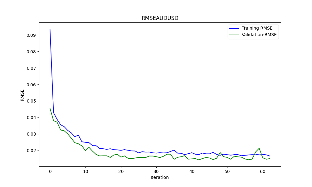
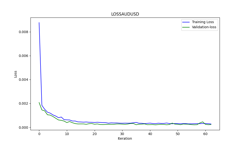
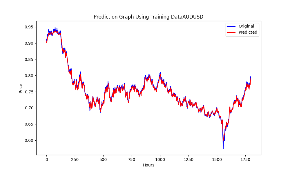
# python libraries
import MetaTrader5 as mt5
import tensorflow as tf
import numpy as np
import pandas as pd
import tf2onnx

# input parameters

inp_history_size = 120

sample_size = 120*20
symbol = "AUDUSD"
optional = "D1"
inp_model_name = str(symbol)+"_"+str(optional)+".onnx" 

if not mt5.initialize():
    print("initialize() failed, error code =",mt5.last_error())
    quit()

# we will save generated onnx-file near the our script to use as resource
from sys import argv
data_path=argv[0]
last_index=data_path.rfind("\\")+1
data_path=data_path[0:last_index]
print("data path to save onnx model",data_path)

# and save to MQL5\Files folder to use as file
terminal_info=mt5.terminal_info()
file_path=terminal_info.data_path+"\\MQL5\\Files\\"
print("file path to save onnx model",file_path)

# set start and end dates for history data
from datetime import timedelta, datetime
#end_date = datetime.now()
end_date = datetime(2023, 1, 1, 0)
start_date = end_date - timedelta(days=inp_history_size*20)

# print start and end dates
print("data start date =",start_date)
print("data end date =",end_date)

# get rates
eurusd_rates = mt5.copy_rates_from(symbol, mt5.TIMEFRAME_D1, end_date, sample_size)

# create dataframe
df = pd.DataFrame(eurusd_rates)

# get close prices only
data = df.filter(['close']).values

# scale data
from sklearn.preprocessing import MinMaxScaler
scaler=MinMaxScaler(feature_range=(0,1))
scaled_data = scaler.fit_transform(data)

# training size is 80% of the data
training_size = int(len(scaled_data)*0.80) 
print("Training_size:",training_size)
train_data_initial = scaled_data[0:training_size,:]
test_data_initial = scaled_data[training_size:,:1]

# split a univariate sequence into samples
def split_sequence(sequence, n_steps):
    X, y = list(), list()
    for i in range(len(sequence)):
       # find the end of this pattern
       end_ix = i + n_steps
       # check if we are beyond the sequence
       if end_ix > len(sequence)-1:
          break
       # gather input and output parts of the pattern
       seq_x, seq_y = sequence[i:end_ix], sequence[end_ix]
       X.append(seq_x)
       y.append(seq_y)
    return np.array(X), np.array(y)

# split into samples
time_step = inp_history_size
x_train, y_train = split_sequence(train_data_initial, time_step)
x_test, y_test = split_sequence(test_data_initial, time_step)

# reshape input to be [samples, time steps, features] which is required for LSTM
x_train =x_train.reshape(x_train.shape[0],x_train.shape[1],1)
x_test = x_test.reshape(x_test.shape[0],x_test.shape[1],1)



# define model
from keras.models import Sequential
from keras.layers import Dense, Activation, Conv1D, MaxPooling1D, Dropout, Flatten, LSTM
from keras.metrics import RootMeanSquaredError as rmse
from tensorflow.keras import callbacks
model = Sequential()
model.add(Conv1D(filters=256, kernel_size=2, activation='relu',padding = 'same',input_shape=(inp_history_size,1)))
model.add(MaxPooling1D(pool_size=2))
model.add(LSTM(100, return_sequences = True))
model.add(Dropout(0.3))
model.add(LSTM(100, return_sequences = False))
model.add(Dropout(0.3))
model.add(Dense(units=1, activation = 'sigmoid'))
model.compile(optimizer='adam', loss= 'mse' , metrics = [rmse()])

# Set up early stopping
early_stopping = callbacks.EarlyStopping(
    monitor='val_loss',
    patience=20,
    restore_best_weights=True,
)

# model training for 300 epochs
history = model.fit(x_train, y_train, epochs = 300 , validation_data = (x_test,y_test), batch_size=32, callbacks=[early_stopping], verbose=2)

# evaluate training data
train_loss, train_rmse = model.evaluate(x_train,y_train, batch_size = 32)
print(f"train_loss={train_loss:.3f}")
print(f"train_rmse={train_rmse:.3f}")

# evaluate testing data
test_loss, test_rmse = model.evaluate(x_test,y_test, batch_size = 32)
print(f"test_loss={test_loss:.3f}")
print(f"test_rmse={test_rmse:.3f}")

# save model to ONNX
output_path = data_path+inp_model_name
onnx_model = tf2onnx.convert.from_keras(model, output_path=output_path)
print(f"saved model to {output_path}")

output_path = file_path+inp_model_name
onnx_model = tf2onnx.convert.from_keras(model, output_path=output_path)
print(f"saved model to {output_path}")

# finish
mt5.shutdown()
#prediction using testing data

#prediction using testing data
test_predict = model.predict(x_test)
print(test_predict)
print("longitud total de la prediccion: ", len(test_predict))
print("longitud total del sample: ", sample_size)

plot_y_test = np.array(y_test).reshape(-1, 1)  # Selecciona solo el último elemento de cada muestra de prueba
plot_y_train = y_train.reshape(-1,1)
train_predict = model.predict(x_train)
#print(plot_y_test)

#calculate metrics
from sklearn import metrics
from sklearn.metrics import r2_score
#transform data to real values
value1=scaler.inverse_transform(plot_y_test)
#print(value1)
# Escala las predicciones inversas al transformarlas a la escala original
value2 = scaler.inverse_transform(test_predict.reshape(-1, 1))
#print(value2)
#calc score
score = np.sqrt(metrics.mean_squared_error(value1,value2))

print("RMSE         : {}".format(score))
print("MSE          :", metrics.mean_squared_error(value1,value2))
print("R2 score     :",metrics.r2_score(value1,value2))


#sumarize model
model.summary()

#Print error
value11=pd.DataFrame(value1)
value22=pd.DataFrame(value2)
#print(value11)
#print(value22)



value111=value11.iloc[:,:]
value222=value22.iloc[:,:]

print("longitud salida (tandas de 1 hora): ",len(value111) )
print("en horas son " + str((len(value111))*60*24)+ " minutos")
print("en horas son " + str(((len(value111)))*60*24/60)+ " horas")
print("en horas son " + str(((len(value111)))*60*24/60/24)+ " dias")


# Calculate error
error = value111 - value222

import matplotlib.pyplot as plt
# Plot error
plt.figure(figsize=(10, 6))
plt.scatter(range(len(error)), error, color='blue', label='Error')
plt.axhline(y=0, color='red', linestyle='--', linewidth=1)  # Línea horizontal en y=0
plt.title('Error de Predicción ' + str(symbol))
plt.xlabel('Índice de la muestra')
plt.ylabel('Error')
plt.legend()
plt.grid(True)
plt.savefig(str(symbol)+str(optional)+'.png') 

rmse_ = format(score)
mse_ = metrics.mean_squared_error(value1,value2)
r2_ = metrics.r2_score(value1,value2)

resultados= [rmse_,mse_,r2_]

# Abre un archivo en modo escritura
with open(str(symbol)+str(optional)+"results.txt", "w") as archivo:
    # Escribe cada resultado en una línea separada
    for resultado in resultados:
        archivo.write(str(resultado) + "\n")

# finish
mt5.shutdown()

#show iteration-rmse graph for training and validation
plt.figure(figsize = (18,10))
plt.plot(history.history['root_mean_squared_error'],label='Training RMSE',color='b')
plt.plot(history.history['val_root_mean_squared_error'],label='Validation-RMSE',color='g')
plt.xlabel("Iteration")
plt.ylabel("RMSE")
plt.title("RMSE" + str(symbol))
plt.legend()
plt.savefig(str(symbol)+str(optional)+'1.png') 

#show iteration-loss graph for training and validation
plt.figure(figsize = (18,10))
plt.plot(history.history['loss'],label='Training Loss',color='b')
plt.plot(history.history['val_loss'],label='Validation-loss',color='g')
plt.xlabel("Iteration")
plt.ylabel("Loss")
plt.title("LOSS" + str(symbol))
plt.legend()
plt.savefig(str(symbol)+str(optional)+'2.png') 

#show actual vs predicted (training) graph
plt.figure(figsize=(18,10))
plt.plot(scaler.inverse_transform(plot_y_train),color = 'b', label = 'Original')
plt.plot(scaler.inverse_transform(train_predict),color='red', label = 'Predicted')
plt.title("Prediction Graph Using Training Data" + str(symbol))
plt.xlabel("Hours")
plt.ylabel("Price")
plt.legend()
plt.savefig(str(symbol)+str(optional)+'3.png') 

#show actual vs predicted (testing) graph
plt.figure(figsize=(18,10))
plt.plot(scaler.inverse_transform(plot_y_test),color = 'b',  label = 'Original')
plt.plot(scaler.inverse_transform(test_predict),color='g', label = 'Predicted')
plt.title("Prediction Graph Using Testing Data" + str(symbol))
plt.xlabel("Hours")
plt.ylabel("Price")
plt.legend()
plt.savefig(str(symbol)+str(optional)+'4.png') 

This .py results, in a ONNX model, and some graphs and values as will be shown, we will need both models chosen from the correlation & cointegration pairs we chosed:

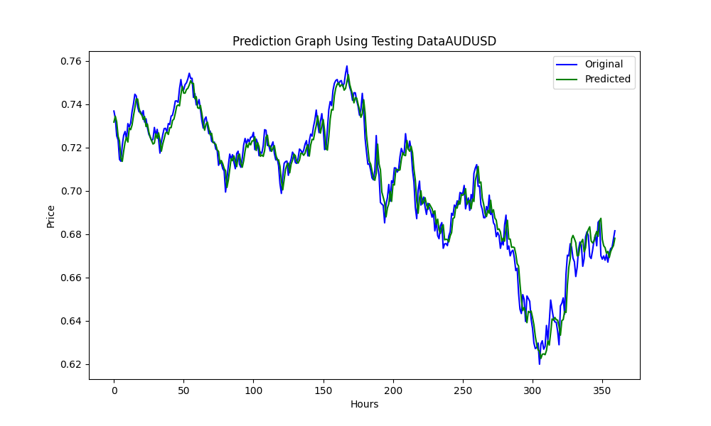
and results

0.005679790676089899
3.226002212419775e-05
0.9670613229880559

that are: RMSE, MSE and R2 respectively.

Back testing with Python

You can use this .py, change the strategy and check results for back testing:

import MetaTrader5 as mt5
import pandas as pd
from scipy.stats import pearsonr
from statsmodels.tsa.stattools import coint
import numpy as np


# Función para la estrategia de Pairs Trading
def pairs_trading_strategy(data0, data1):
    spread = data0 - data1
    short_entry = np.mean(spread) - 2 * np.std(spread)
    short_exit = np.mean(spread)
    long_entry = np.mean(spread) + 2 * np.std(spread)
    long_exit = np.mean(spread)

    positions = []
    for i in range(len(spread)):
        if spread[i] > long_entry and (not positions or positions[-1][1] != 1):
            positions.append((spread[i], 1))
        elif spread[i] < short_entry and (not positions or positions[-1][1] != -1):
            positions.append((spread[i], -1))
        elif spread[i] < long_exit and positions and positions[-1][1] == 1:
            positions.append((spread[i], 0))
        elif spread[i] > short_exit and positions and positions[-1][1] == -1:
            positions.append((spread[i], 0))

    return positions


# Conectar con MetaTrader 5
if not mt5.initialize():
    print("No se pudo inicializar MT5")
    mt5.shutdown()

# Obtener la lista de símbolos
symbols = mt5.symbols_get()
symbols = [s.name for s in symbols if 'EUR' in s.name or 'USD' in s.name]  # Filtrar símbolos

data = {}
for symbol in symbols:
    rates = mt5.copy_rates_from_pos(symbol, mt5.TIMEFRAME_D1, 0, 365)
    if rates is not None:
        df = pd.DataFrame(rates)
        df['time'] = pd.to_datetime(df['time'], unit='s')  # Convertir a datetime
        df.set_index('time', inplace=True)
        data[symbol] = df['close']

mt5.shutdown()

# Identificar pares cointegrados
cointegrated_pairs = []
for i in range(len(symbols)):
    for j in range(i + 1, len(symbols)):
        if symbols[i] in data and symbols[j] in data:
            common_index = data[symbols[i]].index.intersection(data[symbols[j]].index)
            if len(common_index) > 30:
                corr, _ = pearsonr(data[symbols[i]][common_index], data[symbols[j]][common_index])
                if abs(corr) > 0.8:
                    score, p_value, _ = coint(data[symbols[i]][common_index], data[symbols[j]][common_index])
                    if p_value < 0.05:
                        cointegrated_pairs.append((symbols[i], symbols[j], corr, p_value))

print(cointegrated_pairs)

# Ejecutar estrategia de Pairs Trading para pares cointegrados
for sym1, sym2, _, _ in cointegrated_pairs:
    positions = []
    df0 = data[sym1]
    df1 = data[sym2]

    positions = pairs_trading_strategy(df0.values, df1.values)

    print(f'Backtesting completed for pair: {sym1} - {sym2}')
    print('Positions:', positions)

Back testing with MT5 Strategy Tester

Once we have the ONNX models, we can run the EA, I've chosen to use a simple strategy, you can choose what ever strategy you whant/need, and pleased if you can show results and strategy.

When I first did this for me, NZDUSD and AUDUSD where cointegrated and corelated, but at this moment they don't pass the filter (cointegration smaller than 0.05). For teaching purposes and to not need to make the ONNX models again, I will continue with this two symbols.

//+------------------------------------------------------------------+
//|                               Hybrid Arbitrage_Statistic ONNX.mq5|
//|           Copyright 2024, Javier S. Gastón de Iriarte Cabrera. |
//|                      https://www.mql5.com/en/users/jsgaston/news |
//+------------------------------------------------------------------+
#property copyright   "Copyright 2024, Javier S. Gastón de Iriarte Cabrera."
#property link        "https://www.mql5.com/en/users/jsgaston/news"
#property version     "1.00"

#property strict
#include <Trade\Trade.mqh>
input double lotSize = 0.1;
//input double slippage = 3;
input double stopLoss = 1500;
input double takeProfit = 1500;
//input double maxSpreadPoints = 10.0;

#resource "/Files/art/hybrid/NZDUSD_D1.onnx" as uchar ExtModel[]
#resource "/Files/art/hybrid/AUDUSD_D1.onnx" as uchar ExtModel2[]

#define SAMPLE_SIZE 120

string symbol1 = _Symbol;
input string symbol2 = "AUDUSD";
ulong ticket1 = 0;
ulong ticket2 = 0;
input bool isArbitrageActive = true;
CTrade ExtTrade;
double spreads[1000]; // Array para almacenar hasta 1000 spreads
int spreadIndex = 0; // Índice para el próximo spread a almacenar

long     ExtHandle=INVALID_HANDLE;
//int      ExtPredictedClass=-1;
datetime ExtNextBar=0;
datetime ExtNextDay=0;
float    ExtMin=0.0;
float    ExtMax=0.0;


long     ExtHandle2=INVALID_HANDLE;
//int      ExtPredictedClass=-1;
datetime ExtNextBar2=0;
datetime ExtNextDay2=0;
float    ExtMin2=0.0;
float    ExtMax2=0.0;

float predicted=0.0;
float predicted2=0.0;

float   lastPredicted1=0.0;
float   lastPredicted2=0.0;

int Order=0;
//+------------------------------------------------------------------+
//| Expert initialization function                                   |
//+------------------------------------------------------------------+
int OnInit()
  {
   Print("EA de arbitraje ONNX iniciado");

//--- create a model from static buffer
   ExtHandle=OnnxCreateFromBuffer(ExtModel,ONNX_DEFAULT);
   if(ExtHandle==INVALID_HANDLE)
     {
      Print("OnnxCreateFromBuffer error ",GetLastError());
      return(INIT_FAILED);
     }

//--- since not all sizes defined in the input tensor we must set them explicitly
//--- first index - batch size, second index - series size, third index - number of series (only Close)
   const long input_shape[] = {1,SAMPLE_SIZE,1};
   if(!OnnxSetInputShape(ExtHandle,ONNX_DEFAULT,input_shape))
     {
      Print("OnnxSetInputShape error ",GetLastError());
      return(INIT_FAILED);
     }

//--- since not all sizes defined in the output tensor we must set them explicitly
//--- first index - batch size, must match the batch size of the input tensor
//--- second index - number of predicted prices (we only predict Close)
   const long output_shape[] = {1,1};
   if(!OnnxSetOutputShape(ExtHandle,0,output_shape))
     {
      Print("OnnxSetOutputShape error ",GetLastError());
      return(INIT_FAILED);
     }


//--- create a model from static buffer
   ExtHandle2=OnnxCreateFromBuffer(ExtModel2,ONNX_DEFAULT);
   if(ExtHandle2==INVALID_HANDLE)
     {
      Print("OnnxCreateFromBuffer error ",GetLastError());
      return(INIT_FAILED);
     }

//--- since not all sizes defined in the input tensor we must set them explicitly
//--- first index - batch size, second index - series size, third index - number of series (only Close)
   const long input_shape2[] = {1,SAMPLE_SIZE,1};
   if(!OnnxSetInputShape(ExtHandle2,ONNX_DEFAULT,input_shape2))
     {
      Print("OnnxSetInputShape error ",GetLastError());
      return(INIT_FAILED);
     }

//--- since not all sizes defined in the output tensor we must set them explicitly
//--- first index - batch size, must match the batch size of the input tensor
//--- second index - number of predicted prices (we only predict Close)
   const long output_shape2[] = {1,1};
   if(!OnnxSetOutputShape(ExtHandle2,0,output_shape2))
     {
      Print("OnnxSetOutputShape error ",GetLastError());
      return(INIT_FAILED);
     }



   return(INIT_SUCCEEDED);
  }

//+------------------------------------------------------------------+
//| Expert deinitialization function                                 |
//+------------------------------------------------------------------+
void OnDeinit(const int reason)
  {
   if(ExtHandle!=INVALID_HANDLE)
     {
      OnnxRelease(ExtHandle);
      ExtHandle=INVALID_HANDLE;
     }

   if(ExtHandle2!=INVALID_HANDLE)
     {
      OnnxRelease(ExtHandle2);
      ExtHandle2=INVALID_HANDLE;
     }
  }

//+------------------------------------------------------------------+
//| Expert tick function                                             |
//+------------------------------------------------------------------+
void OnTick()
  {
//--- check new day
   if(TimeCurrent()>=ExtNextDay)
     {
      GetMinMax();
      GetMinMax2();
      //--- set next day time
      ExtNextDay=TimeCurrent();
      ExtNextDay-=ExtNextDay%PeriodSeconds(PERIOD_D1);
      ExtNextDay+=PeriodSeconds(PERIOD_D1);
      /*ExtTrade.PositionClose(symbol1);
      ExtTrade.PositionClose(symbol2);
      ticket1 = 0;
      ticket2 = 0;*/
     }

//--- check new bar
   if(TimeCurrent()<ExtNextBar)
     {

      return;
     }
//--- set next bar time
   ExtNextBar=TimeCurrent();
   ExtNextBar-=ExtNextBar%PeriodSeconds();
   ExtNextBar+=PeriodSeconds();
//--- check min and max
   float close=(float)iClose(symbol1,PERIOD_D1,0);
   if(ExtMin>close)
      ExtMin=close;
   if(ExtMax<close)
      ExtMax=close;
   float close2=(float)iClose(symbol2,PERIOD_D1,0);
   if(ExtMin2>close2)
      ExtMin2=close2;
   if(ExtMax2<close2)
      ExtMax2=close2;

   lastPredicted1=predicted;
   lastPredicted2=predicted2;

//--- predict next price
   PredictPrice();
   PredictPrice2();



   if(!isArbitrageActive || ArePositionsOpen())
     {
      Print("Arbitraje inactivo o ya hay posiciones abiertas.");
      return;
     }
   double price1 = SymbolInfoDouble(symbol1, SYMBOL_BID);
   double price2 = SymbolInfoDouble(symbol2, SYMBOL_ASK);
   double currentSpread = MathAbs(price1 - price2);
   Print("current spread ", currentSpread);
   Print("Price1 ",price1);
   Print("Price2 ",price2);
   Print("PricePredicted1 ",predicted);
   Print("PricePredicted2 ",predicted2);
   Print("Last PricePredicted1 ",lastPredicted1);
   Print("Last PricePredicted2 ",lastPredicted2);

   double predictedSpread = MathAbs(predicted - predicted2);
   Print("Predicted spread ", predictedSpread);

   double LastpredictedSpread = MathAbs(lastPredicted1 - lastPredicted2);
   Print("Last Predicted spread ", LastpredictedSpread);

// Almacenar el spread actual en el array y actualizar el índice
   spreads[spreadIndex % 1000] = currentSpread;
   spreadIndex++;

// Verifica si hay suficientes datos para calcular la desviación estándar
   int count = MathMin(spreadIndex, 1000); // Utiliza todos los datos disponibles hasta 1000
   double stdDevSpread = CalculateStdDev(spreads, 0, count);
//Print("StdDevSpread ", stdDevSpread);

// Verifica si el spread es lo suficientemente bajo para el arbitraje
   if(LastpredictedSpread< currentSpread)
     {
      // Inicia el arbitraje si aún no está activo
      if(isArbitrageActive)
        {
         //Print("max spread : ",maxSpreadPoints * _Point);
         double meanSpread = (lastPredicted1 + lastPredicted2) / 2.0;
         Print("mean spread: ",meanSpread);
         double stdDevSpread = CalculateStdDev(spreads, 0, ArraySize(spreads));
         Print("StdDevSpread ", stdDevSpread);
         double shortEntry = meanSpread - 2 * stdDevSpread ;

         double shortExit = meanSpread;
         double longEntry = meanSpread + 2 * stdDevSpread ;

         double longExit = meanSpread;

         Print("Long Entry: ", longEntry, " Short Entry: ", shortEntry);

         // Comprueba si la condición de entrada corta se cumple para el arbitraje
         if(price1 < shortEntry && (ticket1 == 0 || ticket2 == 0))
           {
            Print("Preparando para abrir órdenes");
            Order = 1;


            Print("Error al abrir posiciones de arbitraje: ", GetLastError());
            ticket1 = ExtTrade.PositionOpen(symbol1, ORDER_TYPE_BUY, lotSize, price1, price1 - stopLoss * _Point, price1 + takeProfit * _Point, "Arbitraje");
            ticket2 = ExtTrade.PositionOpen(symbol2, ORDER_TYPE_SELL, lotSize, price2, price2 + stopLoss * _Point, price2 - takeProfit * _Point, "Arbitraje");
            ticket1=0;
            ticket2=0;
           }
         else
            if(price2 < shortEntry && (ticket1 == 0 || ticket2 == 0))
              {
               Print("Preparando para abrir órdenes");
               Order = 2;


               Print("Error al abrir posiciones de arbitraje: ", GetLastError());
               ticket1 = ExtTrade.PositionOpen(symbol1, ORDER_TYPE_SELL, lotSize, price1, price1 + stopLoss * _Point, price1 - takeProfit * _Point, "Arbitraje");
               ticket2 = ExtTrade.PositionOpen(symbol2, ORDER_TYPE_BUY, lotSize, price2, price2 - stopLoss * _Point, price2 + takeProfit * _Point, "Arbitraje");
               ticket1=0;
               ticket2=0;
              }

            else
               if(price1 > longEntry && (ticket1 == 0 || ticket2 == 0))
                 {
                  Print("Preparando para abrir órdenes");
                  Order = 3;


                  Print("Error al abrir posiciones de arbitraje: ", GetLastError());
                  ticket1 = ExtTrade.PositionOpen(symbol1, ORDER_TYPE_SELL, lotSize, price1, price1 + stopLoss * _Point, price1 - takeProfit * _Point, "Arbitraje");
                  ticket2 = ExtTrade.PositionOpen(symbol2, ORDER_TYPE_BUY, lotSize, price2, price2 - stopLoss * _Point, price2 + takeProfit * _Point, "Arbitraje");
                  ticket1=0;
                  ticket2=0;
                 }
               else
                  if(price2 > longEntry && (ticket1 == 0 || ticket2 == 0))
                    {
                     Print("Preparando para abrir órdenes");
                     Order = 4;


                     Print("Error al abrir posiciones de arbitraje: ", GetLastError());

                     ticket1 = ExtTrade.PositionOpen(symbol1, ORDER_TYPE_BUY, lotSize, price1, price1 - stopLoss * _Point, price1 + takeProfit * _Point, "Arbitraje");
                     ticket2 = ExtTrade.PositionOpen(symbol2, ORDER_TYPE_SELL, lotSize, price2, price2 + stopLoss * _Point, price2 - takeProfit * _Point, "Arbitraje");
                     ticket1=0;
                     ticket2=0;
                    }

        }
     }
//+------------------------------------------------------------------+
//|                                                                  |
//+------------------------------------------------------------------+
   double meanSpread = (lastPredicted1 + lastPredicted2) / 2.0;
//Print("mean spread: ",meanSpread);
   double stdDevSpread2 = CalculateStdDev(spreads, 0, ArraySize(spreads));
//Print("StdDevSpread ", stdDevSpread);
   double shortEntry = meanSpread - 2 * stdDevSpread2 ;

   double shortExit = meanSpread;
   double longEntry = meanSpread + 2 * stdDevSpread2 ;

   double longExit = meanSpread;
   if((price2 < longExit && ticket2 != 0 && Order==4) || (price1 > shortExit && ticket1 != 0 && Order==1) || (price2 > shortExit && ticket1 != 0 && Order==2) || (price1 < longExit && ticket2 != 0 && Order==3))
     {
      ExtTrade.PositionClose(ticket1);
      ExtTrade.PositionClose(ticket2);
      ticket1 = 0;
      ticket2 = 0;
      Print("Arbitraje detenido - Cerrando órdenes");
     }

  }

//+------------------------------------------------------------------+
//|                                                                  |
//+------------------------------------------------------------------+
double CalculateStdDev(double &data[], int start, int count)
  {
   double sum = 0;
   double sumSq = 0;
   for(int i = start; i < start + count; i++)
     {
      sum += data[i];
      sumSq += data[i] * data[i];
     }
   double mean = sum / count;
   double variance = (sumSq / count) - (mean * mean);
   return MathSqrt(variance);
  }
//+------------------------------------------------------------------+
//|                                                                  |
//+------------------------------------------------------------------+
bool ArePositionsOpen()
  {
// Check for positions on symbol1
   if(PositionSelect(symbol1) && PositionGetDouble(POSITION_VOLUME) > 0)
      return true;
// Check for positions on symbol2
   if(PositionSelect(symbol2) && PositionGetDouble(POSITION_VOLUME) > 0)
      return true;

   return false;
  }
//+------------------------------------------------------------------+
void PredictPrice(void)
  {
   static vectorf output_data(1);            // vector to get result
   static vectorf x_norm(SAMPLE_SIZE);       // vector for prices normalize

//--- check for normalization possibility
   if(ExtMin>=ExtMax)
     {
      Print("ExtMin>=ExtMax");
      //ExtPredictedClass=-1;
      return;
     }
//--- request last bars
   if(!x_norm.CopyRates(_Symbol,PERIOD_D1,COPY_RATES_CLOSE,1,SAMPLE_SIZE))
     {
      Print("CopyRates ",x_norm.Size());
      //ExtPredictedClass=-1;
      return;
     }
   float last_close=x_norm[SAMPLE_SIZE-1];
//--- normalize prices
   x_norm-=ExtMin;
   x_norm/=(ExtMax-ExtMin);
//--- run the inference
   if(!OnnxRun(ExtHandle,ONNX_NO_CONVERSION,x_norm,output_data))
     {
      Print("OnnxRun");
      //ExtPredictedClass=-1;
      return;
     }
//--- denormalize the price from the output value
   predicted=output_data[0]*(ExtMax-ExtMin)+ExtMin;
//return predicted;
  }
//+------------------------------------------------------------------+
//|                                                                  |
//+------------------------------------------------------------------+
void PredictPrice2(void)
  {
   static vectorf output_data2(1);            // vector to get result
   static vectorf x_norm2(SAMPLE_SIZE);       // vector for prices normalize

//--- check for normalization possibility
   if(ExtMin2>=ExtMax2)
     {
      Print("ExtMin2>=ExtMax2");
      //ExtPredictedClass=-1;
      return;
     }
//--- request last bars
   if(!x_norm2.CopyRates(symbol2,PERIOD_D1,COPY_RATES_CLOSE,1,SAMPLE_SIZE))
     {
      Print("CopyRates ",x_norm2.Size());
      //ExtPredictedClass=-1;
      return;
     }
   float last_close2=x_norm2[SAMPLE_SIZE-1];
//--- normalize prices
   x_norm2-=ExtMin2;
   x_norm2/=(ExtMax2-ExtMin2);
//--- run the inference
   if(!OnnxRun(ExtHandle2,ONNX_NO_CONVERSION,x_norm2,output_data2))
     {
      Print("OnnxRun");
      //ExtPredictedClass=-1;
      return;
     }
//--- denormalize the price from the output value
   predicted2=output_data2[0]*(ExtMax2-ExtMin2)+ExtMin2;
//--- classify predicted price movement
//return predicted2;
  }

//+------------------------------------------------------------------+
//| Get minimal and maximal Close for last 120 days                  |
//+------------------------------------------------------------------+
void GetMinMax(void)
  {
   vectorf close;
   close.CopyRates(_Symbol,PERIOD_D1,COPY_RATES_CLOSE,0,SAMPLE_SIZE);
   ExtMin=close.Min();
   ExtMax=close.Max();
  }

//+------------------------------------------------------------------+
//| Get minimal and maximal Close for last 120 days                  |
//+------------------------------------------------------------------+
void GetMinMax2(void)
  {
   vectorf close2;
   close2.CopyRates(symbol2,PERIOD_D1,COPY_RATES_CLOSE,0,SAMPLE_SIZE);
   ExtMin2=close2.Min();
   ExtMax2=close2.Max();
  }

This are the results for NZDUSD with AUDUSD for 1 minute period time frame with ONNX models of 1 day time frame period with SL 1500 pts and TP of 1500 pts with models that predict from first of January 2023 to first of January 2024 :

To select other pairs to filter, change this line:

symbols = [s.name for s in symbols if s.name.startswith('EUR') or s.name.startswith('USD') or s.name.endswith('USD')]

Case study 2

Arbitrage is very used in stocks trading, this is why I find interesting doing another example with pairs from NASDAQ.

In my case, I changed this line:

symbols = [s.name for s in symbols if s.name.startswith('EUR') or s.name.startswith('USD') or s.name.endswith('USD')]

for this:

# Crea un DataFrame con la información completa de los símbolos
symbols_df = pd.DataFrame([{'Symbol': symbol.name, 'Path': symbol.path} for symbol in all_symbols])

# Filtra adicionalmente para obtener solo los CFDs de NASDAQ
# Asumiendo que los CFDs tienen un identificador único en el 'Path'
nasdaq_group4_df = symbols_df[symbols_df['Path'].str.contains('NASDAQ')]

# Filtra aún más para obtener solo los símbolos que NO contienen '.'
nasdaq_group4_df3 = nasdaq_group4_df[nasdaq_group4_df['Symbol'].str.contains('#')]

nasdaq_group4_df2 = nasdaq_group4_df3[~nasdaq_group4_df3['Symbol'].str.contains('\.')]

# Ahora, obtenemos la lista de símbolos filtrados
filtered_symbols = nasdaq_group4_df2['Symbol'].tolist()
# Descargar datos históricos y almacenar en un diccionario
symbols = filtered_symbols

This where the pairs filtered:

(there where so many pairs cointegrated and corelated, that I had to change the script ( modify the .py to print this in a csv)).

chages:

# Filtrar y guardar solo los pares cointegrados con p-valor menor de 0.05 en un archivo CSV
result_df = pd.DataFrame(cointegrated_pairs, columns=['Symbol1', 'Symbol2', 'Correlation', 'Cointegration P-value'])
result_df.to_csv('cointegrated_pairs.csv', index=False)

# Imprimir el total de pares cointegrados
print(f'Total de pares con fuerte correlación y cointegrados: {len(cointegrated_pairs)}')

This are the pairs filtered from NASDAQ (add excel with results)

For now on, I will continue with Amazon and Netflix with models that predict from first of January 2023 to first of January 2024.

#AMZN   #NFLX   0.966605859     0.021683012

In order to get better results, sample size was multiplied three times more

sample_size = 120*25*3

Results where this:

6.856399020501732
47.010207528337105
0.9395402850007741 

25.975755379462548
674.7398675336775
0.9735838717570285 

With SL of 400 and TP of 800

and finetuning SL's and TP's this is what we ended having with a quick optimization:

Left all scripts and ONNX as the EA's to download so you can methodically && scientifically use this to get the same results. It will be up to you to make new ONNX on the dates you need (remember to change the dates on the training .py's) and also the dates in the Strategy Tester. Example: ONNX models for D1 time periods and 120*3*25 of data can be used max over a year (but if I was you, I would make them each weak or month).

Remember, this is only a strategy with its example, it's not a ready built on bot to use to trade, and you will probably never find one for free in internet.

Conclusion

We've seen how to use correlation and cointegration, to end up having a Pearson's coefficient indicator and an EA for arbitrage trading using predictions. Better results can be obtained when using the correct pairs from the .py filter. You can fine tune the SL's and TP's to achieve better results and make the strategy more complex to get better results. 

Remember to store the ONNX models in the MQL5/Files folder, the mq5 indicator in the Indicator folder and the EA in the Expert Advisors folder (Experts).