Deep Neural Networks (Part VIII). Increasing the classification quality of bagging ensembles
Vladimir Perervenko | 28 September, 2018
Contents
- Introduction
- Preparing Initial Data
- Processing noise samples in the pretrain subset
- Training ensembles of neural network classifiers on denoised initial data and calculating continuous predictions of neural networks on test subsets
- Determining the thresholds for the obtained continuous predictions, converting them into class labels, and calculating metrics for neural networks
- Testing ensembles
- Optimizing hyperparameters of ensembles of neural network classifiers
- Optimizing postprocessing hyperparameters
- Combining several best ensembles into a superensemble as well as their outputs
- Analyzing experimental results
- Conclusion
- Attachments
Introduction
In the previous two articles (1, 2), we created an ensemble of ELM neural network classifiers. That time we discussed how the classification quality could be improved. Among the many possible solutions, two were chosen: reduce the impact of noise samples and select the optimal threshold, by which the continuous predictions of the ensemble's neural networks are converted into class labels. In this article, I propose to experimentally test how the classification quality is affected by:
- data denoising methods,
- threshold types,
- optimization of hyperparameters the ensemble's neural networks and postprocessing.
Then compare the quality of classification obtained by averaging and by a simple majority voting of the superensemble composed of the best ensembles following the optimization results. All computations are performed in the R 3.4.4 environment.
1. Preparing Initial Data
To prepare the initial data, we will use the scripts described previously.
In the first block (Library), load the necessary functions and libraries.
In the second block (prepare), using the quotes with timestamps passed from the terminal, calculate the indicator values (in this case, these are digital filters) and additional variables based on OHLC. Combine this data set into dataframe dt. Then define the parameters of outliers in these data and impute them. Then define the normalization parameters and normalize the data. We get the resulting set of input data DTcap.n.
In the third block (Data X1), generate two sets:
- data1 — contains all 13 indicators with the Data timestamps and the Class target;
- X1 — the same set of predictors but without a timestamp. The target is converted to a numeric value (0, 1).
In the fourth block (Data X2), also generate two sets:
- data2 — contains 7 predictors and a timestamp (Data, CO, HO, LO, HL, dC, dH, dL);
- Х2 — the same predictors but without a timestamp.
#--1--Library-------------
patch <- "C:/Users/Vladimir/Documents/Market/Statya_DARCH2/PartVIII/PartVIII/"
source(file = paste0(patch,"importar.R"))
source(file = paste0(patch,"Library.R"))
source(file = paste0(patch,"FunPrepareData_VII.R"))
source(file = paste0(patch,"FUN_Stacking_VIII.R"))
import_fun(NoiseFiltersR, GE, noise)
#--2-prepare----
evalq({
  dt <- PrepareData(Data, Open, High, Low, Close, Volume)
  DT <- SplitData(dt$features, 4000, 1000, 500, 250, start = 1)
  pre.outl <- PreOutlier(DT$pretrain)
  DTcap <- CappingData(DT, impute = T, fill = T, dither = F, pre.outl = pre.outl)
  meth <- qc(expoTrans, range)# "spatialSign" "expoTrans" "range" "spatialSign",
  preproc <- PreNorm(DTcap$pretrain, meth = meth, rang = c(-0.95, 0.95))
  DTcap.n <- NormData(DTcap, preproc = preproc)
}, env)

#--3-Data X1-------------
evalq({
  subset <- qc(pretrain, train, test, test1)
  foreach(i = 1:length(DTcap.n)) %do% {
    DTcap.n[[i]] ->.;
    dp$select(., Data, ftlm, stlm, rbci, pcci, fars,
              v.fatl, v.satl, v.rftl, v.rstl,v.ftlm,
              v.stlm, v.rbci, v.pcci, Class)} -> data1
  names(data1) <- subset
  X1 <- vector(mode = "list", 4)
  foreach(i = 1:length(X1)) %do% {
    data1[[i]] %>% dp$select(-c(Data, Class)) %>% as.data.frame() -> x
    data1[[i]]$Class %>% as.numeric() %>% subtract(1) -> y
    list(x = x, y = y)} -> X1
  names(X1) <- subset
}, env)
#--4-Data-X2-------------
evalq({
  foreach(i = 1:length(DTcap.n)) %do% {
    DTcap.n[[i]] ->.;
    dp$select(., Data, CO, HO, LO, HL, dC, dH, dL)} -> data2
  names(data2) <- subset
  X2 <- vector(mode = "list", 4)
  foreach(i = 1:length(X2)) %do% {
    data2[[i]] %>% dp$select(-Data) %>% as.data.frame() -> x
    DT[[i]]$dz -> y
    list(x = x, y = y)} -> X2
  names(X2) <- subset
  rm(dt, DT, pre.outl, DTcap, meth, preproc)
}, env)
In the fifth block (bestF), sort the predictors of the Х1 set in ascending order of their importance (orderX1). Select those of them with the coefficient above 0.5 (featureX1). Print the coefficients and names of the selected predictors.
#--5--bestF-----------------------------------
#require(clusterSim)
evalq({
  orderF(x = X1$pretrain$x %>% as.matrix(), type = "metric", s = 1, 4,
         distance =  NULL, # "d1" - Manhattan, "d2" - Euclidean,
         #"d3" - Chebychev (max), "d4" - squared Euclidean,
         #"d5" - GDM1, "d6" - Canberra, "d7" - Bray-Curtis
         method = "kmeans" ,#"kmeans" (default) , "single",
         #"ward.D", "ward.D2", "complete", "average", "mcquitty",
         #"median", "centroid", "pam"
         Index = "cRAND") -> rx1
  rx1$stopri[ ,1] -> orderX1
  featureX1 <- dp$filter(rx1$stopri %>% as.data.frame(), rx1$stopri[ ,2] > 0.5) %>%
    dp$select(V1) %>% unlist() %>% unname()
}, env)
print(env$rx1$stopri)
      [,1]      [,2]
 [1,]    6 1.0423206
 [2,]   12 1.0229287
 [3,]    7 0.9614459
 [4,]   10 0.9526798
 [5,]    5 0.8884596
 [6,]    1 0.8055126
 [7,]    3 0.7959655
 [8,]   11 0.7594309
 [9,]    8 0.6960105
[10,]    2 0.6626440
[11,]    4 0.4905196
[12,]    9 0.3554887
[13,]   13 0.2269289
colnames(env$X1$pretrain$x)[env$featureX1]
[1] "v.fatl" "v.rbci" "v.satl" "v.ftlm" "fars"   "ftlm"   "rbci"   "v.stlm" "v.rftl"
[10] "stlm"
The same calculations are performed for the second data set Х2. We obtain orderX2 and featureX2.
evalq({
  orderF(x = X2$pretrain$x %>% as.matrix(), type = "metric", s = 1, 4,
         distance =  NULL, # "d1" - Manhattan, "d2" - Euclidean,
         #"d3" - Chebychev (max), "d4" - squared Euclidean,
         #"d5" - GDM1, "d6" - Canberra, "d7" - Bray-Curtis
         method = "kmeans" ,#"kmeans" (default) , "single",
         #"ward.D", "ward.D2", "complete", "average", "mcquitty",
         #"median", "centroid", "pam"
         Index = "cRAND") -> rx2
  rx2$stopri[ ,1] -> orderX2
  featureX2 <- dp$filter(rx2$stopri %>% as.data.frame(), rx2$stopri[ ,2] > 0.5) %>%
    dp$select(V1) %>% unlist() %>% unname()
}, env)
print(env$rx2$stopri)
     [,1]      [,2]
[1,]    1 1.6650259
[2,]    5 1.6636689
[3,]    3 0.7751799
[4,]    2 0.7751351
[5,]    6 0.5692846
[6,]    7 0.5496889
[7,]    4 0.4970882
colnames(env$X2$pretrain$x)[env$featureX2]
[1] "CO" "dC" "LO" "HO" "dH" "dL"
This completes the preparation of the initial data for the experiments. We have prepared two data sets X1/data1, X2/data2 and predictors orderX1, orderX2 ranked by importance. All the above scripts are located in the Prepare_VIII.R file.
2. Processing noise samples in the pretrain subset
Many authors of articles, including myself, devoted their publications to the filtering of noise predictors. Here I propose to explore another, equally important, but less used feature — the identification and processing of noise samples in data sets. So why are some examples in data sets considered noise and what methods can be used to process them? I will try to explain.
Thus, we are faced with the task of classification, while we have a training set of predictors and a target. The target is considered to correspond well to the internal structure of the training set. But in reality, the data structure of the predictors set is much more complicated than the proposed structure of the target. It turns out that the set contains examples that correspond to the target well, while there are some that do not correspond to it at all, greatly distorting the model when learning. As a result, this leads to a decrease in the quality of the model classification. The approaches to identifying and processing the noise samples have already been considered in detail. Here we check how the classification quality is affected by three processing methods:
- correction of the mistakenly labeled examples;
- removing them from the set;
- allocating them to a separate class.
The noise samples will be identified and processed using the NoiseFiltersR::GE() function. It looks for the noise samples and modifies their labels (corrects erroneous labeling). Examples that cannot be relabeled are removed. The identified noise samples can also be removed from the set manually, or moved to a separate class, assigning a new label to them. All the calculations above are performed on the 'pretrain' subset, since it will be used for training the ensemble. See the result of the function:
#---------------------------
import_fun(NoiseFiltersR, GE, noise)
#-----------------------
evalq({
  out <- noise(x = data1[[1]] %>% dp$select(-Data))
  summary(out, explicit = TRUE)
}, env)
Filter GE applied to dataset

Call:
GE(x = data1[[1]] %>% dp$select(-Data))

Parameters:
k: 5
kk: 3

Results:
Number of removed instances: 0 (0 %)
Number of repaired instances: 819 (20.46988 %)

Explicit indexes for removed instances:
.......
Output structure of the out function:
> str(env$out)
List of 7
 $ cleanData :'data.frame':     4001 obs. of  14 variables:
  ..$ ftlm  : num [1:4001] 0.293 0.492 0.47 0.518 0.395 ...
  ..$ stlm  : num [1:4001] 0.204 0.185 0.161 0.153 0.142 ...
  ..$ rbci  : num [1:4001] -0.0434 0.1156 0.1501 0.25 0.248 ...
  ..$ pcci  : num [1:4001] -0.0196 -0.0964 -0.4455 0.2685 -0.0349 ...
  ..$ fars  : num [1:4001] 0.208 0.255 0.246 0.279 0.267 ...
  ..$ v.fatl: num [1:4001] 0.4963 0.4635 0.0842 0.3707 0.0542 ...
  ..$ v.satl: num [1:4001] -0.0146 0.0248 -0.0353 0.1797 0.1205 ...
  ..$ v.rftl: num [1:4001] -0.2695 -0.0809 0.1752 0.3637 0.5305 ...
  ..$ v.rstl: num [1:4001] 0.398 0.362 0.386 0.374 0.357 ...
  ..$ v.ftlm: num [1:4001] 0.5244 0.4039 -0.0296 0.1088 -0.2299 ...
  ..$ v.stlm: num [1:4001] -0.275 -0.226 -0.285 -0.11 -0.148 ...
  ..$ v.rbci: num [1:4001] 0.5374 0.4811 0.0978 0.2992 -0.0141 ...
  ..$ v.pcci: num [1:4001] -0.8779 -0.0706 -0.3125 0.6311 -0.2712 ...
  ..$ Class : Factor w/ 2 levels "-1","1": 2 2 2 2 2 1 1 1 1 1 ...
 $ remIdx    : int(0)
 $ repIdx    : int [1:819] 16 27 30 31 32 34 36 38 46 58 ...
 $ repLab    : Factor w/ 2 levels "-1","1": 2 2 2 1 1 2 2 2 1 1 ...
 $ parameters:List of 2
  ..$ k : num 5
  ..$ kk: num 3
 $ call      : language GE(x = data1[[1]] %>% dp$select(-Data))
 $ extraInf  : NULL
 - attr(*, "class")= chr "filter"
Where:
- out$cleanData — the data set after correcting the labeling of the noise samples,
- out$remIdx — indexes of the removed samples (none in our example),
- out$repIdx — indexes of the samples with targets relabeled,
- out$repLab — new labels of these noise samples. Thus, we can remove them from the set or assign a new label to them using out$repIdx.
Once the indexes of the noise samples are determined, prepare four data sets for training the ensembles combined into the denoiseX1pretrain structure.
- denoiseX1pretrain$origin — the original pretraining set;
- denoiseX1pretrain$repaired — data set with the labeling of the noise samples corrected;
- denoiseX1pretrain$removed — data set with the noise samples removed;
- denoiseX1pretrain$relabeled — data set with the noise samples assigned a new label (i.e., the target now has three classes).
#--2-Data Xrepair-------------
#library(NoiseFiltersR)
evalq({
  out <- noise(x = data1$pretrain %>% dp$select(-Data))
  Yrelab <- X1$pretrain$y
  Yrelab[out$repIdx] <- 2L
  X1rem <- data1$pretrain[-out$repIdx, ] %>% dp$select(-Data)
  denoiseX1pretrain <- list(origin = list(x = X1$pretrain$x,  y = X1$pretrain$y),
                            repaired = list(x = X1$pretrain$x, y = out$cleanData$Class %>%
                                             as.numeric() %>% subtract(1)),
                             removed = list(x = X1rem %>% dp$select(-Class),
                                          y = X1rem$Class %>% as.numeric() %>% subtract(1)),
                             relabeled = list(x = X1$pretrain$x, y = Yrelab))
  rm(out, Yrelab, X1rem)
}, env)
The subsets denoiseX1pretrain$origin|repaired|relabeled have the identical predictors х, but the target у is different in every set. Let us have a look at their structure:
#-------------------------
env$denoiseX1pretrain$repaired$x  %>% str()
'data.frame':   4001 obs. of  13 variables:
 $ ftlm  : num  0.293 0.492 0.47 0.518 0.395 ...
 $ stlm  : num  0.204 0.185 0.161 0.153 0.142 ...
 $ rbci  : num  -0.0434 0.1156 0.1501 0.25 0.248 ...
 $ pcci  : num  -0.0196 -0.0964 -0.4455 0.2685 -0.0349 ...
 $ fars  : num  0.208 0.255 0.246 0.279 0.267 ...
 $ v.fatl: num  0.4963 0.4635 0.0842 0.3707 0.0542 ...
 $ v.satl: num  -0.0146 0.0248 -0.0353 0.1797 0.1205 ...
 $ v.rftl: num  -0.2695 -0.0809 0.1752 0.3637 0.5305 ...
 $ v.rstl: num  0.398 0.362 0.386 0.374 0.357 ...
 $ v.ftlm: num  0.5244 0.4039 -0.0296 0.1088 -0.2299 ...
 $ v.stlm: num  -0.275 -0.226 -0.285 -0.11 -0.148 ...
 $ v.rbci: num  0.5374 0.4811 0.0978 0.2992 -0.0141 ...
 $ v.pcci: num  -0.8779 -0.0706 -0.3125 0.6311 -0.2712 ...
env$denoiseX1pretrain$relabeled$x  %>% str()
'data.frame':   4001 obs. of  13 variables:
 $ ftlm  : num  0.293 0.492 0.47 0.518 0.395 ...
 $ stlm  : num  0.204 0.185 0.161 0.153 0.142 ...
 $ rbci  : num  -0.0434 0.1156 0.1501 0.25 0.248 ...
 $ pcci  : num  -0.0196 -0.0964 -0.4455 0.2685 -0.0349 ...
 $ fars  : num  0.208 0.255 0.246 0.279 0.267 ...
 $ v.fatl: num  0.4963 0.4635 0.0842 0.3707 0.0542 ...
 $ v.satl: num  -0.0146 0.0248 -0.0353 0.1797 0.1205 ...
 $ v.rftl: num  -0.2695 -0.0809 0.1752 0.3637 0.5305 ...
 $ v.rstl: num  0.398 0.362 0.386 0.374 0.357 ...
 $ v.ftlm: num  0.5244 0.4039 -0.0296 0.1088 -0.2299 ...
 $ v.stlm: num  -0.275 -0.226 -0.285 -0.11 -0.148 ...
 $ v.rbci: num  0.5374 0.4811 0.0978 0.2992 -0.0141 ...
 $ v.pcci: num  -0.8779 -0.0706 -0.3125 0.6311 -0.2712 ...
env$denoiseX1pretrain$repaired$y  %>% table()
.
   0    1
1888 2113
env$denoiseX1pretrain$removed$y  %>% table()
.
   0    1
1509 1673
env$denoiseX1pretrain$relabeled$y  %>% table()
.
   0    1    2
1509 1673  819
Since the number of samples in the set denoiseX1pretrain$removed has changed, let us check how the significance of the predictors has changed:
evalq({
  orderF(x = denoiseX1pretrain$removed$x %>% as.matrix(),
         type = "metric", s = 1, 4,
         distance =  NULL, # "d1" - Manhattan, "d2" - Euclidean,
         #"d3" - Chebychev (max), "d4" - squared Euclidean,
         #"d5" - GDM1, "d6" - Canberra, "d7" - Bray-Curtis
         method = "kmeans" ,#"kmeans" (default) , "single",
         #"ward.D", "ward.D2", "complete", "average", "mcquitty",
         #"median", "centroid", "pam"
         Index = "cRAND") -> rx1rem
  rx1rem$stopri[ ,1] -> orderX1rem
  featureX1rem <- dp$filter(rx1rem$stopri %>% as.data.frame(),
                            rx1rem$stopri[ ,2] > 0.5) %>%
    dp$select(V1) %>% unlist() %>% unname()
}, env)
print(env$rx1rem$stopri)
     [,1]      [,2]
 [1,]    6 1.0790642
 [2,]   12 1.0320772
 [3,]    7 0.9629750
 [4,]   10 0.9515987
 [5,]    5 0.8426669
 [6,]    1 0.8138830
 [7,]    3 0.7934568
 [8,]   11 0.7682185
 [9,]    8 0.6720211
[10,]    2 0.6355753
[11,]    4 0.5159589
[12,]    9 0.3670544
[13,]   13 0.2170575
colnames(env$X1$pretrain$x)[env$featureX1rem]
[1] "v.fatl" "v.rbci" "v.satl" "v.ftlm" "fars"   "ftlm"   "rbci"   "v.stlm" "v.rftl"
[10] "stlm"   "pcci"
The order and composition of the best predictors has changed. This will need to be considered when training ensembles.
So, we have 4 subsets ready: denoiseX1pretrain$origin, repaired, removed, relabeled. They will be used for training the ELM ensembles. Scripts for denoising the data are located in the Denoise.R file. The structure of the initial data Х1 and denoiseX1pretrain looks as follows:
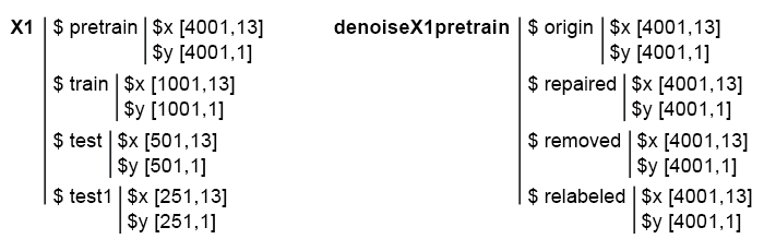
Fig. 1. The structure of the initial data.
3. Training ensembles of neural network classifiers on denoised initial data and calculating continuous predictions of neural networks on test subsets
Let us write a function for training the ensemble and receiving predictions which will later serve as the input data for the trainable combiner in the stacking ensemble.
Such calculations have already been performed in the previous article, therefore, their details will not be discussed. In short:
- in block 1 (Input), define the constants;
- in block 2 (createEns), define the function CreateEns(), that would create an ensemble of individual neural network classifiers with constant parameters and reproducible initialization;
- in block 3 (GetInputData), the GetInputData() function calculates the predictions of three subsets Х1$ train/test/test1 using the ensemble Ens.
#--1--Input-------------
evalq({
  #type of activation function.
  Fact <- c("sig", #: sigmoid
            "sin", #: sine
            "radbas", #: radial basis
            "hardlim", #: hard-limit
            "hardlims", #: symmetric hard-limit
            "satlins", #: satlins
            "tansig", #: tan-sigmoid
            "tribas", #: triangular basis
            "poslin", #: positive linear
            "purelin") #: linear
  n <- 500
  r = 7L
  SEED <- 12345
  #--2-createENS----------------------
  createEns <- function(r = 7L, nh = 5L, fact = 7L, X, Y){
    Xtrain <- X[ , featureX1]
    k <- 1
    rng <- RNGseq(n, SEED)
    #---creste Ensemble---
    Ens <- foreach(i = 1:n, .packages = "elmNN") %do% {
      rngtools::setRNG(rng[[k]])
      idx <- rminer::holdout(Y, ratio = r/10, mode = "random")$tr
      k <- k + 1
      elmtrain(x = Xtrain[idx, ], y = Y[idx], nhid = nh, actfun = Fact[fact])
    }
    return(Ens)
  }
  #--3-GetInputData -FUN-----------
  GetInputData <- function(Ens, X, Y){
    #---predict-InputPretrain--------------
    Xtrain <- X[ ,featureX1]
    k <- 1
    rng <- RNGseq(n, SEED)
    #---create Ensemble---
    foreach(i = 1:n, .packages = "elmNN", .combine = "cbind") %do% {
      rngtools::setRNG(rng[[k]])
      idx <- rminer::holdout(Y, ratio = r/10, mode = "random")$tr
      k <- k + 1
      predict(Ens[[i]], newdata = Xtrain[-idx, ])
    } %>% unname() -> InputPretrain
    #---predict-InputTrain--
    Xtest <- X1$train$x[ , featureX1]
    foreach(i = 1:n, .packages = "elmNN", .combine = "cbind") %do% {
      predict(Ens[[i]], newdata = Xtest)
    } -> InputTrain #[ ,n]
    #---predict--InputTest----
    Xtest1 <- X1$test$x[ , featureX1]
    foreach(i = 1:n, .packages = "elmNN", .combine = "cbind") %do% {
      predict(Ens[[i]], newdata = Xtest1)
    } -> InputTest #[ ,n]
    #---predict--InputTest1----
    Xtest2 <- X1$test1$x[ , featureX1]
    foreach(i = 1:n, .packages = "elmNN", .combine = "cbind") %do% {
      predict(Ens[[i]], newdata = Xtest2)
    } -> InputTest1 #[ ,n]
    #---res-------------------------
    return(list(InputPretrain = InputPretrain,
                InputTrain = InputTrain,
                InputTest = InputTest,
                InputTest1 = InputTest1))
  }
}, env)
We already have the denoiseX1pretrain set with four groups of data for training ensembles: original (origin), with corrected labeling (repaired), with removed (removed) and relabeled (relabeled) noise samples. After training the ensemble on each of these groups of data, we obtain four ensembles. Using these ensembles with the GetInputData() function, we obtain four groups of predictions in three subsets: train, test and test1. Below are the scripts separately for each ensemble in the expanded form (only for debugging and ease of understanding).
#---4--createEns--origin--------------
evalq({
  Ens.origin <- vector(mode = "list", n)
  res.origin <- vector("list", 4)
  x <- denoiseX1pretrain$origin$x %>% as.matrix()
  y <- denoiseX1pretrain$origin$y
  createEns(r = 7L, nh = 5L, fact = 7L, X = x, Y = y) -> Ens.origin
  GetInputData(Ens = Ens.origin, X = x, Y = y) -> res.origin
}, env)
#---4--createEns--repaired--------------
evalq({
  Ens.repaired <- vector(mode = "list", n)
  res.repaired <- vector("list", 4)
  x <- denoiseX1pretrain$repaired$x %>% as.matrix()
  y <- denoiseX1pretrain$repaired$y
  createEns(r = 7L, nh = 5L, fact = 7L,  X = x, Y = y) -> Ens.repaired
  GetInputData(Ens = Ens.repaired, X = x, Y = y) -> res.repaired
}, env)
#---4--createEns--removed--------------
evalq({
  Ens.removed <- vector(mode = "list", n)
  res.removed <- vector("list", 4)
  x <- denoiseX1pretrain$removed$x %>% as.matrix()
  y <- denoiseX1pretrain$removed$y
  createEns(r = 7L, nh = 5L, fact = 7L, X = x, Y = y) -> Ens.removed
  GetInputData(Ens = Ens.removed,  X = x, Y = y) -> res.removed
}, env)
#---4--createEns--relabeled--------------
evalq({
  Ens.relab <- vector(mode = "list", n)
  res.relab <- vector("list", 4)
  x <- denoiseX1pretrain$relabeled$x %>% as.matrix()
  y <- denoiseX1pretrain$relabeled$y
  createEns(r = 7L, nh = 5L, fact = 7L, X = x, Y = y) -> Ens.relab
  GetInputData(Ens = Ens.relab,  X = x, Y = y) -> res.relab
}, env)
The structure of the ensemble predictions results is shown below:
> env$res.origin %>% str()
List of 4
 $ InputPretrain: num [1:1201, 1:500] 0.747 0.774 0.733 0.642 0.28 ...
 $ InputTrain   : num [1:1001, 1:500] 0.742 0.727 0.731 0.66 0.642 ...
 $ InputTest    : num [1:501, 1:500] 0.466 0.446 0.493 0.594 0.501 ...
 $ InputTest1   : num [1:251, 1:500] 0.093 0.101 0.391 0.547 0.416 ...
> env$res.repaired %>% str()
List of 4
 $ InputPretrain: num [1:1201, 1:500] 0.815 0.869 0.856 0.719 0.296 ...
 $ InputTrain   : num [1:1001, 1:500] 0.871 0.932 0.889 0.75 0.737 ...
 $ InputTest    : num [1:501, 1:500] 0.551 0.488 0.516 0.629 0.455 ...
 $ InputTest1   : num [1:251, 1:500] -0.00444 0.00877 0.35583 0.54344 0.40121 ...
> env$res.removed %>% str()
List of 4
 $ InputPretrain: num [1:955, 1:500] 0.68 0.424 0.846 0.153 0.242 ...
 $ InputTrain   : num [1:1001, 1:500] 0.864 0.981 0.784 0.624 0.713 ...
 $ InputTest    : num [1:501, 1:500] 0.755 0.514 0.439 0.515 0.156 ...
 $ InputTest1   : num [1:251, 1:500] 0.105 0.108 0.511 0.622 0.339 ...
> env$res.relab %>% str()
List of 4
 $ InputPretrain: num [1:1201, 1:500] 1.11 1.148 1.12 1.07 0.551 ...
 $ InputTrain   : num [1:1001, 1:500] 1.043 0.954 1.088 1.117 1.094 ...
 $ InputTest    : num [1:501, 1:500] 0.76 0.744 0.809 0.933 0.891 ...
 $ InputTest1   : num [1:251, 1:500] 0.176 0.19 0.615 0.851 0.66 ...
Let us see how the distribution of these outputs/inputs looks like. See the first 10 outputs of the InputTrain[ ,1:10] sets:
#------Ris InputTrain------
par(mfrow = c(2, 2), mai = c(0.3, 0.3, 0.4, 0.2))
boxplot(env$res.origin$InputTrain[ ,1:10], horizontal = T, main = "res.origin$InputTrain[ ,1:10]")
abline(v = c(0, 0.5, 1.0), col = 2)
boxplot(env$res.repaired$InputTrain[ ,1:10], horizontal = T, main = "res.repaired$InputTrain[ ,1:10]")
abline(v = c(0, 0.5, 1.0), col = 2)
boxplot(env$res.removed$InputTrain[ ,1:10], horizontal = T, main = "res.removed$InputTrain[ ,1:10]")
abline(v = c(0, 0.5, 1.0), col = 2)
boxplot(env$res.relab$InputTrain[ ,1:10], horizontal = T, main = "res.relab$InputTrain[ ,1:10]")
abline(v = c(0, 0.5, 1.0), col = 2)
par(mfrow = c(1, 1))

Fig. 2. Distribution of predictions of the InputTrain outputs using four different ensembles.
See the 10 first outputs of the InputTest[ ,1:10] sets:
#------Ris InputTest------
par(mfrow = c(2, 2), mai = c(0.3, 0.3, 0.4, 0.2), las = 1)

boxplot(env$res.origin$InputTest[ ,1:10], horizontal = T, main = "res.origin$InputTest[ ,1:10]")
abline(v = c(0, 0.5, 1.0), col = 2)
boxplot(env$res.repaired$InputTest[ ,1:10], horizontal = T, main = "res.repaired$InputTest[ ,1:10]")
abline(v = c(0, 0.5, 1.0), col = 2)
boxplot(env$res.removed$InputTest[ ,1:10], horizontal = T, main = "res.removed$InputTest[ ,1:10]")
abline(v = c(0, 0.5, 1.0), col = 2)
boxplot(env$res.relab$InputTest[ ,1:10], horizontal = T, main = "res.relab$InputTest[ ,1:10]")
abline(v = c(0, 0.5, 1.0), col = 2)
par(mfrow = c(1, 1))

Fig. 3. Distribution of predictions of the InputTest outputs using four different ensembles.
See the 10 first outputs of the InputTest1[ ,1:10] sets:
#------Ris InputTest1------
par(mfrow = c(2, 2), mai = c(0.3, 0.3, 0.4, 0.2))
boxplot(env$res.origin$InputTest1[ ,1:10], horizontal = T, main = "res.origin$InputTest1[ ,1:10]")
abline(v = c(0, 0.5, 1.0), col = 2)
boxplot(env$res.repaired$InputTest1[ ,1:10], horizontal = T, main = "res.repaired$InputTest1[ ,1:10]")
abline(v = c(0, 0.5, 1.0), col = 2)
boxplot(env$res.removed$InputTest1[ ,1:10], horizontal = T, main = "res.removed$InputTest1[ ,1:10]")
abline(v = c(0, 0.5, 1.0), col = 2)
boxplot(env$res.relab$InputTest1[ ,1:10], horizontal = T, main = "res.relab$InputTest1[ ,1:10]")
abline(v = c(0, 0.5, 1.0), col = 2)
par(mfrow = c(1, 1))

Fig. 4. Distribution of predictions of the InputTest1 outputs using four different ensembles.
Distribution of all predictions differs greatly from the predictions obtained from the data normalized by the SpatialSign method in the previous experiments. You can experiment with different normalization methods on your own.
After calculating the prediction of subsets X1$train/test/test1 using each ensemble, we obtain four groups of data — res.origin, res.repaired, res.removed and res.relab, with distributions shown in Figures 2 — 4.
Let us determine the classification quality of each ensemble, converting the continuous predictions into class labels.
4. Determining the thresholds for the obtained continuous predictions, converting them into class labels, and calculating metrics for neural networks
To convert the continuous data into class labels, one or several thresholds of division into these classes are used. The continuous predictions of the InputTrain sets, obtained from the fifth neural network of all ensembles, look as follows:

Fig. 5. Continuous predictions of the fifth neural network of various ensembles.
As you can see, the graphs of continuous prediction of the origin, repaired, relabeled models are similar in shape, but have a different range. The line of the removed model's prediction is considerably different in shape.
To simplify the subsequent calculations, collect all models and their predictions in one structure predX1. To do this, write a compact function that will repeat all calculations in a cycle. There is the script and a picture of the predX1 structure:
library("doFuture")
#---predX1------------------
evalq({
  group <- qc(origin, repaired, removed, relabeled)
  predX1 <- vector("list", 4)
  foreach(i = 1:4, .packages = "elmNN") %do% {
    x <- denoiseX1pretrain[[i]]$x %>% as.matrix()
    y <- denoiseX1pretrain[[i]]$y
    SEED = 12345
    createEns(r = 7L, nh = 5L, fact = 7L, X = x, Y = y) -> ens
    GetInputData(Ens = ens, X = x, Y = y) -> pred
    return(list(ensemble = ens, pred = pred))
  } -> predX1
  names(predX1) <- group
}, env)
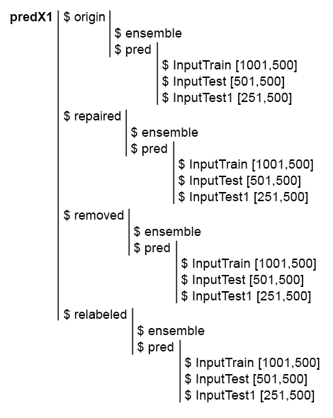
Fig. 6. Structure of the predX1 set
Remember that to obtain the metrics of the ensemble's prediction quality, two operations need to be performed: pruning and averaging (or simple majority voting). For pruning, it is necessary to convert all outputs of the ensemble's every neural network from the continuous form into class labels. Then define the metrics of each neural network and select a certain number of them with the best scores. Then average the continuous predictions of these best neural networks and obtain a continuous average prediction of the ensemble. Once more, define the threshold, convert the averaged prediction into class labels and calculate the final scores of the ensemble's classification quality.
Thus, it is necessary to convert the continuous prediction into class labels twice. The conversion thresholds at these two stages can either be the same or different. Which variants of thresholds can be used?
- The default threshold. In this case, it is equal to 0.5.
- Threshold equal to the median. I think it is more reliable. But the median can be determined only on the validation set, while it can be applied only when testing the subsequent subsets. For example, we define the thresholds on the InputTrain subset, which will later be used on the InputTest and InputTest1 subsets.
- Threshold optimized for various criteria. For example, it can be the minimum classification error, the maximum accuracy "1", or "0", etc. The optimal thresholds are always determined on the InputTrain subset, and used on the InputTest and InputTest1 subsets.
- When averaging the outputs of the best neural networks, calibration can be used. Some authors write that only well-calibrated outputs can be averaged. Confirming this statement is beyond the scope of this article.
The optimal threshold will be determined using the InformationValue::optimalCutoff() function. It is described in detail in the package.
To determine the thresholds for points 1 and 2, additional calculations are not required. To calculate the optimal thresholds for point 3, let us write the function GetThreshold().
#--function-------------------------
evalq({
  import_fun("InformationValue", optimalCutoff, CutOff)
  import_fun("InformationValue", youdensIndex, th_youdens)
  GetThreshold <- function(X, Y, type){
    switch(type,
           half = 0.5,
           med = median(X),
           mce = CutOff(Y, X, "misclasserror"),
           both = CutOff(Y, X,"Both"),
            CutOff(Y, X, "Ones"),
           zeros = CutOff(Y, X, "Zeros")
    )
  }
}, env)
Only the first four types of thresholds described in this function (half, med, mce, both) will be calculated. The first two are the half and median thresholds. The mce threshold provides the minimum classification error, the both threshold — the maximum value of the coefficient youdensIndex = (sensitivity + specificity —1). The calculation order will be as follows:
1. In the predX1 set, calculate the four types of thresholds for each of 500 neural networks of the ensemble on the InputTrain subset, separately in each group of data (origin, repaired, removed and relabeled).
2. Then, using these thresholds, convert the continuous predictions of all neural network ensembles in all subsets (train|test|test1) into classes and determine the average values F1. We obtain four groups of metrics containing three subsets each. Below is a step-by-step script for the origin group.
Define 4 types of thresholds on the predX1$origin$pred$InputTrain subset:
#--threshold--train--origin--------
evalq({
  Ytest = X1$train$y
  Ytest1 = X1$test$y
  Ytest2 = X1$test1$y
  testX1 <- vector("list", 4)
  names(testX1) <- group
  type <- qc(half, med, mce, both)
  registerDoFuture()
  cl <- makeCluster(4)
  plan(cluster, workers = cl)
  foreach(i = 1:4, .combine = "cbind") %dopar% {# type
     foreach(j = 1:500, .combine = "c") %do% {
        GetThreshold(predX1$origin$pred$InputTrain[ ,j], Ytest, type[i])
     }
  }  -> testX1$origin$Threshold
  stopCluster(cl)
  dimnames(testX1$origin$Threshold) <- list(NULL,type)
  }, env)
We use two nested loops in each calculation. In the outer loop, select the threshold type, create a cluster, and parallelize the calculation to 4 cores. In the inner loop, iterate over the InputTrain predictions of each of 500 neural networks comprising the ensemble. 4 types of thresholds are defined for each one. The structure of the obtained data will be as follows:
> env$testX1$origin$Threshold %>% str()
 num [1:500, 1:4] 0.5 0.5 0.5 0.5 0.5 0.5 0.5 0.5 0.5 0.5 ...
 - attr(*, "dimnames")=List of 2
  ..$ : NULL
  ..$ : chr [1:4] "half" "med" "mce" "both"
> env$testX1$origin$Threshold %>% head()
     half       med       mce      both
[1,]  0.5 0.5033552 0.3725180 0.5125180
[2,]  0.5 0.4918041 0.5118821 0.5118821
[3,]  0.5 0.5005034 0.5394191 0.5394191
[4,]  0.5 0.5138439 0.4764055 0.5164055
[5,]  0.5 0.5241393 0.5165478 0.5165478
[6,]  0.5 0.4673319 0.4508287 0.4608287
Using the obtained thresholds, covert the continuous predictions of the origin group of the subsets train, test and test1 into class labels and calculate the metrics (mean(F1)).
#--train--------------------
evalq({
  foreach(i = 1:4, .combine = "cbind") %do% {# type
    foreach(j = 1:500, .combine = "c") %do% {
      ifelse(predX1$origin$pred$InputTrain[ ,j] > testX1$origin$Threshold[j, i], 1, 0) ->.;
      Evaluate(actual = Ytest, predicted = .)$Metrics$F1 %>% mean()
    }
  } -> testX1$origin$InputTrainScore
  dimnames(testX1$origin$InputTrainScore)[[2]] <- type
}, env)
#--test-----------------------------
evalq({
  foreach(i = 1:4, .combine = "cbind") %do% {# type
    foreach(j = 1:500, .combine = "c") %do% {
      ifelse(predX1$origin$pred$InputTest[ ,j] > testX1$origin$Threshold[j, i], 1, 0) ->.;
      Evaluate(actual = Ytest1, predicted = .)$Metrics$F1 %>% mean()
    }
  } -> testX1$origin$InputTestScore
  dimnames(testX1$origin$InputTestScore)[[2]] <- type
}, env)
#--test1-----------------------------
evalq({
  foreach(i = 1:4, .combine = "cbind") %do% {
    foreach(j = 1:500, .combine = "c") %do% {
      ifelse(predX1$origin$pred$InputTest1[ ,j] > testX1$origin$Threshold[j, i], 1, 0) ->.;
      Evaluate(actual = Ytest2, predicted = .)$Metrics$F1 %>% mean()
    }
  } -> testX1$origin$InputTest1Score
  dimnames(testX1$origin$InputTest1Score)[[2]] <- type
}, env)
See the distribution of metrics in the origin group and three of its subsets. The script below for the origin group:
k <- 1L #origin
# k <- 2L #repaired
# k <- 3L #removed
# k <- 4L #relabeling
par(mfrow = c(1,4), mai = c(0.3, 0.3, 0.4, 0.2))
boxplot(env$testX1[[k]]$Threshold, horizontal = F,
        main = paste0(env$group[k],"$$Threshold"),
        col = c(2,4,5,6))
abline(h = c(0, 0.5, 0.7), col = 2)
boxplot(env$testX1[[k]]$InputTrainScore, horizontal = F,
        main = paste0(env$group[k],"$$InputTrainScore"),
        col = c(2,4,5,6))
abline(h = c(0, 0.5, 0.7), col = 2)
boxplot(env$testX1[[k]]$InputTestScore, horizontal = F,
        main = paste0(env$group[k],"$$InputTestScore"),
        col = c(2,4,5,6))
abline(h = c(0, 0.5, 0.7), col = 2)
boxplot(env$testX1[[k]]$InputTest1Score, horizontal = F,
        main = paste0(env$group[k],"$$InputTest1Score"),
        col = c(2,4,5,6))
abline(h = c(0, 0.5, 0.7), col = 2)
par(mfrow = c(1, 1))

Fig. 7. Distribution of thresholds and metrics in the origin group
The visualization showed that using "med" as the threshold for the origin group of data does not give a visible improvement in quality compared to the "half" threshold.
Calculate all 4 types of thresholds in all groups (be prepared for it to take quite a lot of time and memory).
library("doFuture")
#--threshold--train---------
evalq({
  k <- 1L #origin
  #k <- 2L #repaired
  #k <- 3L #removed
  #k <- 4L #relabeling
  type <- qc(half, med, mce, both)
  Ytest = X1$train$y
  Ytest1 = X1$test$y
  Ytest2 = X1$test1$y
  registerDoFuture()
  cl <- makeCluster(4)
  plan(cluster, workers = cl)
  while (k <= 4) { # group
    foreach(i = 1:4, .combine = "cbind") %dopar% {# type
      foreach(j = 1:500, .combine = "c") %do% {
        GetThreshold(predX1[[k]]$pred$InputTrain[ ,j], Ytest, type[i])
      }
    }  -> testX1[[k]]$Threshold
    dimnames(testX1[[k]]$Threshold) <- list(NULL,type)
    k <- k + 1
  }
  stopCluster(cl)
}, env)
Using the obtained thresholds, calculate the metrics in all groups and subsets:
#--train--------------------
evalq({
  k <- 1L #origin
  #k <- 2L #repaired
  #k <- 3L #removed
  #k <- 4L #relabeling
  while (k <= 4) {
    foreach(i = 1:4, .combine = "cbind") %do% {
      foreach(j = 1:500, .combine = "c") %do% {
        ifelse(predX1[[k]]$pred$InputTrain[ ,j] > testX1[[k]]$Threshold[j, i], 1, 0) ->.;
        Evaluate(actual = Ytest, predicted = .)$Metrics$F1 %>% mean()
      }
    } -> testX1[[k]]$InputTrainScore
    dimnames(testX1[[k]]$InputTrainScore)[[2]] <- type
    k <- k + 1
  }
}, env)
#--test-----------------------------
evalq({
  k <- 1L #origin
  #k <- 2L #repaired
  #k <- 3L #removed
  #k <- 4L #relabeling
  while (k <= 4) {
    foreach(i = 1:4, .combine = "cbind") %do% {
      foreach(j = 1:500, .combine = "c") %do% {
        ifelse(predX1[[k]]$pred$InputTest[ ,j] > testX1[[k]]$Threshold[j, i], 1, 0) ->.;
        Evaluate(actual = Ytest1, predicted = .)$Metrics$F1 %>% mean()
      }
    } -> testX1[[k]]$InputTestScore
    dimnames(testX1[[k]]$InputTestScore)[[2]] <- type
    k <- k + 1
  }
}, env)
#--test1-----------------------------
evalq({
  k <- 1L #origin
  #k <- 2L #repaired
  #k <- 3L #removed
  #k <- 4L #relabeling
  while (k <= 4) {
    foreach(i = 1:4, .combine = "cbind") %do% {
      foreach(j = 1:500, .combine = "c") %do% {
        ifelse(predX1[[k]]$pred$InputTest1[ ,j] > testX1[[k]]$Threshold[j, i], 1, 0) ->.;
        Evaluate(actual = Ytest2, predicted = .)$Metrics$F1 %>% mean()
      }
    } -> testX1[[k]]$InputTest1Score
    dimnames(testX1[[k]]$InputTest1Score)[[2]] <- type
    k <- k + 1
  }
}, env)
To each group of data, we added metrics of each of the ensemble's 500 neural networks with four different thresholds on three subsets.
Let us see how the metrics are distributed in each group and subset. The script is provided for the repaired subset. It is similar for other groups, only the group number changes. For clarity, the graphs of all groups will be presented in one.
# k <- 1L #origin
 k <- 2L #repaired
# k <- 3L #removed
# k <- 4L #relabeling
par(mfrow = c(1,4), mai = c(0.3, 0.3, 0.4, 0.2))
boxplot(env$testX1[[k]]$Threshold, horizontal = F,
        main = paste0(env$group[k],"$$Threshold"),
        col = c(2,4,5,6))
abline(h = c(0, 0.5, 0.7), col = 2)
boxplot(env$testX1[[k]]$InputTrainScore, horizontal = F,
        main = paste0(env$group[k],"$$InputTrainScore"),
        col = c(2,4,5,6))
abline(h = c(0, 0.5, 0.7), col = 2)
boxplot(env$testX1[[k]]$InputTestScore, horizontal = F,
        main = paste0(env$group[k],"$$InputTestScore"),
        col = c(2,4,5,6))
abline(h = c(0, 0.5, 0.7), col = 2)
boxplot(env$testX1[[k]]$InputTest1Score, horizontal = F,
        main = paste0(env$group[k],"$$InputTest1Score"),
        col = c(2,4,5,6))
abline(h = c(0, 0.5, 0.7), col = 2)
par(mfrow = c(1, 1))

Fig. 8. Distribution graphs of prediction metrics of the ensemble's each neural network in three groups of data with three subsets and four different thresholds.
Common in all groups:
- metrics of the test subset (InputTestScore) are much better than metrics of the validation set (InputTrainScore);
- metrics of the second test subset (InputTest1Score) are noticeably worse than metrics of the first test subset;
- threshold of type "half" shows results not worse than others on all subsets, except relabeled.
5. Testing ensembles
5.1. Determining 7 neural networks with the best metrics in each ensemble and in each group of data in the InputTrain subset
Perform pruning. In each group of data of the testX1 subset, it is necessary to select 7 InputTrainScore values with the largest values of the mean F1. Their indexes will be the indexes of the best neural networks in the ensemble. The script is given below, and can also be found in the Test.R file.
#--bestNN----------------------------------------
evalq({
  nb <- 3L
  k <- 1L
while (k <= 4) {
  foreach(j = 1:4, .combine = "cbind") %do% {
    testX1[[k]]$InputTrainScore[ ,j] %>% order(decreasing = TRUE) %>% head(2*nb + 1)
  } -> testX1[[k]]$bestNN
  dimnames(testX1[[k]]$bestNN) <- list(NULL, type)
  k <- k + 1
  }
}, env)
We obtained indexes of the neural networks with the best scores in four groups of data (origin, repaired, removed, relabeled). Let us take a closer look at them and compare how much these best neural networks differ depending on the group of data and threshold type.
> env$testX1$origin$bestNN
     half med mce both
[1,]  415  75 415  415
[2,]  191 190 220  220
[3,]  469 220 191  191
[4,]  220 469 469  469
[5,]  265 287  57  444
[6,]  393 227 393   57
[7,]   75 322 444  393
> env$testX1$repaired$bestNN
     half med mce both
[1,]  393 393 154  154
[2,]  415  92 205  205
[3,]  205 154 220  220
[4,]  462 190 393  393
[5,]  435 392 287  287
[6,]  392 220  90   90
[7,]  265 287 415  415
> env$testX1$removed$bestNN
     half med mce both
[1,]  283 130 283  283
[2,]  207 110 300  300
[3,]  308 308 110  110
[4,]  159 134 192  130
[5,]  382 207 207  192
[6,]  192 283 130  308
[7,]  130 114 134  207
env$testX1$relabeled$bestNN
     half med mce both
[1,]  234 205 205  205
[2,]   69 287 469  469
[3,]  137 191 287  287
[4,]  269  57 191  191
[5,]  344 469 415  415
[6,]  164  75 444  444
[7,]  184 220  57   57
You can see that the indexes of neural networks with the "mce" and "both" threshold types coincide very often.
5.2. Averaging continuous predictions of these 7 best neural networks.
After choosing the 7 best neural networks, average them in each group of data, in subsets InputTrain, InputTest, InputTest1 and by each threshold type. Script for processing the InputTrain subset in 4 groups:
#--Averaging--train------------------------
evalq({
  k <- 1L
  while (k <= 4) {# group
    foreach(j = 1:4, .combine = "cbind") %do% {# type
      bestNN <- testX1[[k]]$bestNN[ ,j]
      predX1[[k]]$pred$InputTrain[ ,bestNN] %>%
        apply(1, function(x) sum(x)) %>%
        divide_by((2*nb + 1))
    } -> testX1[[k]]$TrainYpred
    dimnames(testX1[[k]]$TrainYpred) <- list(NULL, paste0("Y.aver_", type))
    k <- k + 1
  }
}, env)
Let us take a look at the structure and statistical scores of the obtained averaged continuous predictions in the data group repaired:
> env$testX1$repaired$TrainYpred %>% str()
 num [1:1001, 1:4] 0.849 0.978 0.918 0.785 0.814 ...
 - attr(*, "dimnames")=List of 2
  ..$ : NULL
  ..$ : chr [1:4] "Y.aver_half" "Y.aver_med" "Y.aver_mce" "Y.aver_both"
> env$testX1$repaired$TrainYpred %>% summary()
  Y.aver_half        Y.aver_med        Y.aver_mce       Y.aver_both
 Min.   :-0.2202   Min.   :-0.4021   Min.   :-0.4106   Min.   :-0.4106
 1st Qu.: 0.3348   1st Qu.: 0.3530   1st Qu.: 0.3512   1st Qu.: 0.3512
 Median : 0.5323   Median : 0.5462   Median : 0.5462   Median : 0.5462
 Mean   : 0.5172   Mean   : 0.5010   Mean   : 0.5012   Mean   : 0.5012
 3rd Qu.: 0.7227   3rd Qu.: 0.7153   3rd Qu.: 0.7111   3rd Qu.: 0.7111
 Max.   : 1.1874   Max.   : 1.0813   Max.   : 1.1039   Max.   : 1.1039
The statistics of the last two threshold types is identical here as well. Here are the scripts for the two remaining subsets InputTest, InputTest1:
#--Averaging--test------------------------
evalq({
  k <- 1L
  while (k <= 4) {# group
    foreach(j = 1:4, .combine = "cbind") %do% {# type
      bestNN <- testX1[[k]]$bestNN[ ,j]
      predX1[[k]]$pred$InputTest[ ,bestNN] %>%
        apply(1, function(x) sum(x)) %>%
        divide_by((2*nb + 1))
    } -> testX1[[k]]$TestYpred
    dimnames(testX1[[k]]$TestYpred) <- list(NULL, paste0("Y.aver_", type))
    k <- k + 1
  }
}, env)
#--Averaging--test1------------------------
evalq({
  k <- 1L
  while (k <= 4) {# group
    foreach(j = 1:4, .combine = "cbind") %do% {# type
      bestNN <- testX1[[k]]$bestNN[ ,j]
      predX1[[k]]$pred$InputTest1[ ,bestNN] %>%
        apply(1, function(x) sum(x)) %>%
        divide_by((2*nb + 1))
    } -> testX1[[k]]$Test1Ypred
    dimnames(testX1[[k]]$Test1Ypred) <- list(NULL, paste0("Y.aver_", type))
    k <- k + 1
  }
}, env)
Let us take a look at the statistics of the InputTest subset of the repaired data group:
> env$testX1$repaired$TestYpred %>% summary()
  Y.aver_half        Y.aver_med        Y.aver_mce       Y.aver_both
 Min.   :-0.1524   Min.   :-0.5055   Min.   :-0.5044   Min.   :-0.5044
 1st Qu.: 0.2888   1st Qu.: 0.3276   1st Qu.: 0.3122   1st Qu.: 0.3122
 Median : 0.5177   Median : 0.5231   Median : 0.5134   Median : 0.5134
 Mean   : 0.5114   Mean   : 0.4976   Mean   : 0.4946   Mean   : 0.4946
 3rd Qu.: 0.7466   3rd Qu.: 0.7116   3rd Qu.: 0.7149   3rd Qu.: 0.7149
 Max.   : 1.1978   Max.   : 1.0428   Max.   : 1.0722   Max.   : 1.0722
The statistics of the last two threshold types is identical here too.
5.3. Defining the thresholds for the averaged continuous predictions
Now we have averaged predictions of each ensemble. They need to be converted into class labels and the final metrics of quality for all data groups and threshold types. To do this, similar to the previous calculations, determine the best thresholds using only the InputTrain subsets. The script provided below calculates the thresholds in each group and in each subset:
#-th_aver------------------------------
evalq({
  k <- 1L #origin
  #k <- 2L #repaired
  #k <- 3L #removed
  #k <- 4L #relabeling
  type <- qc(half, med, mce, both)
  Ytest = X1$train$y
  Ytest1 = X1$test$y
  Ytest2 = X1$test1$y
  while (k <= 4) { # group
    foreach(j = 1:4, .combine = "cbind") %do% {# type subset
      foreach(i = 1:4, .combine = "c") %do% {# type threshold
        GetThreshold(testX1[[k]]$TrainYpred[ ,j], Ytest, type[i])
      }
    }  -> testX1[[k]]$th_aver
    dimnames(testX1[[k]]$th_aver) <- list(type, colnames(testX1[[k]]$TrainYpred))
    k <- k + 1
  }
}, env)
5.4. Converting the averaged continuous predictions of the ensembles into class labels and calculating the metrics of the ensembles on the InputTrain, InputTest and InputTest1 subsets of all data groups.
With the th_aver thresholds calculated above, determine the metrics:
#---Metrics--train-------------------------------------
evalq({
  k <- 1L #origin
  #k <- 2L #repaired
  #k <- 3L #removed
  #k <- 4L #relabeling
  type <- qc(half, med, mce, both)
  while (k <= 4) { # group
    foreach(j = 1:4, .combine = "cbind") %do% {# type subset
      foreach(i = 1:4, .combine = "c") %do% {# type threshold
        ifelse(testX1[[k]]$TrainYpred[ ,j] > testX1[[k]]$th_aver[i,j], 1, 0) -> clAver
        Evaluate(actual = Ytest, predicted = clAver)$Metrics$F1 %>%
          mean() %>% round(3)
      }
    }  -> testX1[[k]]$TrainScore
    dimnames(testX1[[k]]$TrainScore) <- list(type, colnames(testX1[[k]]$TrainYpred))
    k <- k + 1
  }
}, env)
#---Metrics--test-------------------------------------
evalq({
  k <- 1L #origin
  #k <- 2L #repaired
  #k <- 3L #removed
  #k <- 4L #relabeling
  type <- qc(half, med, mce, both)
  while (k <= 4) { # group
    foreach(j = 1:4, .combine = "cbind") %do% {# type subset
      foreach(i = 1:4, .combine = "c") %do% {# type threshold
        ifelse(testX1[[k]]$TestYpred[ ,j] > testX1[[k]]$th_aver[i,j], 1, 0) -> clAver
        Evaluate(actual = Ytest1, predicted = clAver)$Metrics$F1 %>%
          mean() %>% round(3)
      }
    }  -> testX1[[k]]$TestScore
    dimnames(testX1[[k]]$TestScore) <- list(type, colnames(testX1[[k]]$TestYpred))
    k <- k + 1
  }
}, env)
#---Metrics--test1-------------------------------------
evalq({
  k <- 1L #origin
  #k <- 2L #repaired
  #k <- 3L #removed
  #k <- 4L #relabeling
  type <- qc(half, med, mce, both)
  while (k <= 4) { # group
    foreach(j = 1:4, .combine = "cbind") %do% {# type subset
      foreach(i = 1:4, .combine = "c") %do% {# type threshold
        ifelse(testX1[[k]]$Test1Ypred[ ,j] > testX1[[k]]$th_aver[i,j], 1, 0) -> clAver
        Evaluate(actual = Ytest2, predicted = clAver)$Metrics$F1 %>%
          mean() %>% round(3)
      }
    }  -> testX1[[k]]$Test1Score
    dimnames(testX1[[k]]$Test1Score) <- list(type, colnames(testX1[[k]]$Test1Ypred))
    k <- k + 1
  }
}, env)
Create a summary table and analyze the obtained metrics. Let us start with the origin group (its noise samples were not processed in any way). We are looking for the scores TestScore and Test1Score. The scores of the TestTrain subset are indicative, they are needed for comparison with the test scores:
> env$testX1$origin$TrainScore
     Y.aver_half Y.aver_med Y.aver_mce Y.aver_both
half       0.711      0.708      0.712       0.712
med        0.711      0.713      0.707       0.707
mce        0.712      0.704      0.717       0.717
both       0.711      0.706      0.717       0.717
> env$testX1$origin$TestScore
     Y.aver_half Y.aver_med Y.aver_mce Y.aver_both
half       0.750      0.738      0.745       0.745
med        0.748      0.742      0.746       0.746
mce        0.742      0.720      0.747       0.747
both       0.748      0.730      0.747       0.747
> env$testX1$origin$Test1Score
     Y.aver_half Y.aver_med Y.aver_mce Y.aver_both
half       0.735      0.732      0.716       0.716
med        0.733      0.753      0.745       0.745
mce        0.735      0.717      0.716       0.716
both       0.733      0.750      0.716       0.716
What does the proposed table show?
The best result of 0.750 in TestScore was shown by the variant with the "half" threshold in both transformations (both when pruning and averaging). However, the quality drops to 0.735 in the Test1Score subset.
A more stable result of ~0.745 in both subsets are shown by the threshold variants (med, mce, both) when pruning and med when averaging.
See the next data group — repaired (with the corrected labeling of the noise samples):
> env$testX1$repaired$TrainScore
     Y.aver_half Y.aver_med Y.aver_mce Y.aver_both
half       0.713      0.711      0.717       0.717
med        0.709      0.709      0.713       0.713
mce        0.728      0.714      0.709       0.709
both       0.728      0.711      0.717       0.717
> env$testX1$repaired$TestScore
     Y.aver_half Y.aver_med Y.aver_mce Y.aver_both
half       0.759      0.761      0.756       0.756
med        0.754      0.748      0.747       0.747
mce        0.758      0.755      0.743       0.743
both       0.758      0.732      0.754       0.754
> env$testX1$repaired$Test1Score
     Y.aver_half Y.aver_med Y.aver_mce Y.aver_both
half       0.719      0.744      0.724       0.724
med        0.738      0.748      0.744       0.744
mce        0.697      0.720      0.677       0.677
both       0.697      0.743      0.731       0.731
The best result displayed in the table is 0.759 in the half/half combination. A more stable result of ~0.750 in both subsets are shown by the threshold variants (half, med, mce, both) when pruning and med when averaging.
See the next data group — removed (with the noise samples removed from the set):
> env$testX1$removed$TrainScore
     Y.aver_half Y.aver_med Y.aver_mce Y.aver_both
half       0.713      0.720      0.724       0.718
med        0.715      0.717      0.715       0.717
mce        0.721      0.722      0.725       0.723
both       0.721      0.720      0.725       0.723
> env$testX1$removed$TestScore
     Y.aver_half Y.aver_med Y.aver_mce Y.aver_both
half       0.761      0.769      0.761       0.751
med        0.752      0.749      0.760       0.752
mce        0.749      0.755      0.753       0.737
both       0.749      0.736      0.753       0.760
> env$testX1$removed$Test1Score
     Y.aver_half Y.aver_med Y.aver_mce Y.aver_both
half       0.712      0.732      0.716       0.720
med        0.729      0.748      0.740       0.736
mce        0.685      0.724      0.721       0.685
both       0.685      0.755      0.721       0.733
Analyze the table. The best result of 0.769 in TestScore was shown by the variant with the med/half thresholds. However, the quality drops to 0.732 in the Test1Score subset. For the TestScore subset, the best combination of thresholds when pruning (half, med, mce, both) and half when averaging produces the best scores of all groups.
See the last data group — relabeled (with the noise samples isolated to a separate class):
> env$testX1$relabeled$TrainScore
     Y.aver_half Y.aver_med Y.aver_mce Y.aver_both
half       0.672      0.559      0.529       0.529
med        0.715      0.715      0.711       0.711
mce        0.712      0.715      0.717       0.717
both       0.710      0.718      0.720       0.720
> env$testX1$relabeled$TestScore
     Y.aver_half Y.aver_med Y.aver_mce Y.aver_both
half       0.719      0.572      0.555       0.555
med        0.736      0.748      0.746       0.746
mce        0.739      0.747      0.745       0.745
both       0.710      0.756      0.754       0.754
> env$testX1$relabeled$Test1Score
     Y.aver_half Y.aver_med Y.aver_mce Y.aver_both
half       0.664      0.498      0.466       0.466
med        0.721      0.748      0.740       0.740
mce        0.739      0.732      0.716       0.716
both       0.734      0.737      0.735       0.735
The best results for this group are produced by the following combination of thresholds: (med, mce, both) when pruning and both or med when averaging.
Keep in mind that you can get values different from mine.
The figure below shows the data structure of testX1 after all the above calculations:
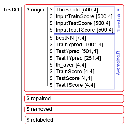
Fig. 9. The data structure of testX1.
6. Optimizing hyperparameters of ensembles of neural network classifiers
All the previous calculations have been carried out on ensembles with the same hyperparameters of neural networks, set based on personal experience. As you may know, the hyperparameters of neural networks, like other models, need to be optimized for a specific data set to obtain better results. For training, we use the denoised data separated into 4 groups (origin, repaired, removed and relabeled). Therefore, it is necessary to obtain optimal hyperparameters of the ensemble's neural networks precisely for these sets. All questions regarding the Bayesian optimization have been thoroughly discussed in the previous article, so their details will not be considered here.
4 hyperparameters of neural networks will be optimized:
- the number of predictors — numFeature = c(3L, 13L) in the range from 3 to 13;
- the percentage of samples used in training — r = c(1L, 10L) in the range from 10 % to 100%;
- the number of neurons in the hidden layer — nh = c(1L, 51L) in the range from 1 to 51;
- type of the activation function — fact = c(1L, 10L) index in the list of activation functions Fact.
Set the constants:
##===OPTIM===============================
evalq({
  #type of activation function.
  Fact <- c("sig", #: sigmoid
            "sin", #: sine
            "radbas", #: radial basis
            "hardlim", #: hard-limit
            "hardlims", #: symmetric hard-limit
            "satlins", #: satlins
            "tansig", #: tan-sigmoid
            "tribas", #: triangular basis
            "poslin", #: positive linear
            "purelin") #: linear
  bonds <- list(
    numFeature = c(3L, 13L),
    r = c(1L, 10L),
    nh = c(1L, 51L),
    fact = c(1L, 10L)
  )
}, env)
Write a fitness function that will return the quality indicator Score = meаn(F1) and the ensemble's prediction in class labels. Pruning (selection of the best neural networks in the ensemble) and averaging of the continuous prediction will be performed using the same threshold = 0.5. It proved to be a very good option earlier — at least for the first approximation. Here is the script:
#---Fitnes -FUN-----------
evalq({
  n <- 500
  numEns <- 3
  # SEED <- c(12345, 1235809)
  fitnes <- function(numFeature, r, nh, fact){
    bestF <- orderX %>% head(numFeature)
    k <- 1
    rng <- RNGseq(n, SEED)
    #---train---
    Ens <- foreach(i = 1:n, .packages = "elmNN") %do% {
      rngtools::setRNG(rng[[k]])
      idx <- rminer::holdout(Ytrain, ratio = r/10, mode = "random")$tr
      k <- k + 1
      elmtrain(x = Xtrain[idx, bestF], y = Ytrain[idx],
               nhid = nh, actfun = Fact[fact])
    }
    #---predict---
    foreach(i = 1:n, .packages = "elmNN", .combine = "cbind") %do% {
      predict(Ens[[i]], newdata = Xtest[ , bestF])
    } -> y.pr #[ ,n]
    #---best---
    foreach(i = 1:n, .combine = "c") %do% {
      ifelse(y.pr[ ,i] > 0.5, 1, 0) -> Ypred
      Evaluate(actual = Ytest, predicted = Ypred)$Metrics$F1 %>%
        mean()
    } -> Score
    Score %>% order(decreasing = TRUE) %>% head((numEns*2 + 1)) -> bestNN
    #---test-aver--------
    foreach(i = 1:n, .packages = "elmNN", .combine = "+") %:%
      when(i %in% bestNN) %do% {
        predict(Ens[[i]], newdata = Xtest1[ , bestF])} %>%
      divide_by(length(bestNN)) -> ensPred
    ifelse(ensPred > 0.5, 1, 0) -> ensPred
    Evaluate(actual = Ytest1, predicted = ensPred)$Metrics$F1 %>%
      mean() %>% round(3) -> Score
    return(list(Score = Score, Pred = ensPred))
  }
}, env)
The SEED variable commented out has two values. This is necessary for checking the impact of this parameter on the result experimentally. I have performed the optimization with the same initial data and parameters, but with two different values of SEED. The best result was shown by SEED = 1235809. This value will be used in the scripts below. But the obtained hyperparameters and classification quality scores will be provided for both values of SEED. You can experiment with other values.
Let us check if the fitness function works, how long one pass of its calculations takes and see the result:
evalq({
   Ytrain <- X1$pretrain$y
   Ytest <- X1$train$y
   Ytest1 <- X1$test$y
   Xtrain <- X1$pretrain$x
   Xtest <- X1$train$x
   Xtest1 <- X1$test$x
   orderX <- orderX1
   SEED <- 1235809
  system.time(
    res <- fitnes(numFeature = 10, r = 7, nh = 5, fact = 2)
  )
 }, env)
user  system elapsed
   5.89    0.00    5.99
env$res$Score
[1] 0.741
Below is the script for optimizing the hyperparameters of neural networks successively for each group of denoised data. Use 20 points of the starting random initialization and 20 subsequent iterations.
#---Optim Ensemble-----
library(rBayesianOptimization)
evalq({
  Ytest <- X1$train$y
  Ytest1 <- X1$test$y
  Xtest <- X1$train$x
  Xtest1 <- X1$test$x
  orderX <- orderX1
  SEED <- 1235809
  OPT_Res <- vector("list", 4)
  foreach(i = 1:4) %do% {
    Xtrain <- denoiseX1pretrain[[i]]$x
    Ytrain <- denoiseX1pretrain[[i]]$y
    BayesianOptimization(fitnes, bounds = bonds,
                                  init_grid_dt = NULL, init_points = 20,
                                  n_iter = 20, acq = "ucb", kappa = 2.576,
                                  eps = 0.0, verbose = TRUE,
                                  maxit = 100, control = c(100, 50, 8))
  } -> OPT_Res1
  group <- qc(origin, repaired, removed, relabeled)
  names(OPT_Res1) <- group
}, env)
Once you start the execution of the script, be patient for about half an hour (it depends on your hardware). Sort the obtained Score values in descending order and choose the three best ones. These scores are assigned to the variables best.res (for SEED = 12345) and best.res1 (for SEED = 1235809).
#---OptPar------
evalq({
  foreach(i = 1:4) %do% {
    OPT_Res[[i]] %$% History %>% dp$arrange(desc(Value)) %>% head(3)
  } -> best.res
  names(best.res) <- group
}, env)
evalq({
  foreach(i = 1:4) %do% {
     OPT_Res1[[i]] %$% History %>% dp$arrange(desc(Value)) %>% head(3)
  } -> best.res1
  names(best.res1) <- group
}, env)
See the best.res scores:
env$best.res
# $origin
#    Round numFeature r nh fact Value
# 1     39         10 7 20    2 0.769
# 2     12          6 4 38    2 0.766
# 3     38          4 3 15    2 0.766

#
# $repaired
#    Round numFeature  r nh fact Value
# 1      5         10  5 20    7 0.767
# 2      7          5  2 36    9 0.766
# 3     28          5 10  6    8 0.766

#
# $removed
#    Round numFeature  r nh fact Value
# 1      1         11  6 44    9 0.764
# 2      8          8  6 26    7 0.764
# 3     19         12  1 40    5 0.763

#
# $relabeled
#    Round numFeature  r nh fact Value
# 1     24          9 10  1   10 0.746
# 2      7          9  9  2    8 0.745
# 3     32          4  1  1   10 0.738
The same for the best.res1 scores:
> env$best.res1
$origin
  Round numFeature r nh fact Value
1    19          8 3 41    2 0.777
2    32          8 1 33    2 0.777
3    23          6 1 35    1 0.770

$repaired
  Round numFeature r nh fact Value
1    26          9 4 17    3 0.772
2    33         11 9 30    9 0.771
3    38          5 4 17    2 0.770

$removed
  Round numFeature r nh fact Value
1    30          5 4 17    2 0.770
2     8          8 2 13    6 0.769
3    32          5 3 22    7 0.766

$relabeled
  Round numFeature r nh fact Value
1    34         12 5  8    9 0.777
2    33          9 5  4    9 0.763
3    36         12 7  4    9 0.760
As you can see, these results look better. For comparison, you can print not the first three results, but ten: the differences will be even more noticeable.
Each optimization run will generate different hyperparameter values and results. The hyperparameters can be optimized using different initial RNG settings, as well as with a specific starting initialization.
Let us collect the best hyperparameters of the ensembles' neural networks for 4 data groups. They will be needed later for creating ensembles with optimal hyperparameters.
#---best.param-------------------
evalq({
  foreach(i = 1:4, .combine = "rbind") %do% {
    OPT_Res1[[i]]$Best_Par %>% unname()
  } -> best.par1
  dimnames(best.par1) <- list(group, qc(numFeature, r, nh, fact))
}, env)
The hyperparameters:
> env$best.par1
          numFeature r nh fact
origin             8 3 41    2
repaired           9 4 17    3
removed            5 4 17    2
relabeled         12 5  8    9
All scripts from this script are available in the Optim_VIII.R file.
7. Optimizing postprocessing hyperparameters (thresholds for pruning and averaging)
Optimization of the neural networks' hyperparameters provides a small increase in the classification quality. As proven earlier, the combination of threshold types when pruning and averaging has a stronger impact on the classification quality.
We have already optimized the hyperparameters with a constant combination of thresholds half/half. Perhaps this combination is not optimal. Let us repeat the optimization with two additional optimized parameters th1 = c(1L, 2L)) — threshold type when pruning the ensemble (selecting the best neural networks) — and th2 = c(1L, 4L) — threshold type when converting the averaged prediction of the ensemble into class labels. Define the constants and the value ranges of the hyperparameters to be optimized.
##===OPTIM===============================
evalq({
  #type of activation function.
  Fact <- c("sig", #: sigmoid
            "sin", #: sine
            "radbas", #: radial basis
            "hardlim", #: hard-limit
            "hardlims", #: symmetric hard-limit
            "satlins", #: satlins
            "tansig", #: tan-sigmoid
            "tribas", #: triangular basis
            "poslin", #: positive linear
            "purelin") #: linear
  bonds_m <- list(
    numFeature = c(3L, 13L),
    r = c(1L, 10L),
    nh = c(1L, 51L),
    fact = c(1L, 10L),
    th1 = c(1L, 2L),
    th2 = c(1L, 4L)
  )
}, env)
On to the fitness function. It was slightly modified: added two formal parameters th1, th2. In the function body and in the 'best' block, calculate the threshold depending on th1. In the 'test-average' block, determine the threshold using the GetThreshold() function depending on the threshold type th2.
#---Fitnes -FUN-----------
evalq({
  n <- 500L
  numEns <- 3L
  # SEED <- c(12345, 1235809)
  fitnes_m <- function(numFeature, r, nh, fact, th1, th2){
    bestF <- orderX %>% head(numFeature)
    k <- 1L
    rng <- RNGseq(n, SEED)
    #---train---
    Ens <- foreach(i = 1:n, .packages = "elmNN") %do% {
      rngtools::setRNG(rng[[k]])
      idx <- rminer::holdout(Ytrain, ratio = r/10, mode = "random")$tr
      k <- k + 1
      elmtrain(x = Xtrain[idx, bestF], y = Ytrain[idx],
               nhid = nh, actfun = Fact[fact])
    }
    #---predict---
    foreach(i = 1:n, .packages = "elmNN", .combine = "cbind") %do% {
      predict(Ens[[i]], newdata = Xtest[ , bestF])
    } -> y.pr #[ ,n]
    #---best---
    ifelse(th1 == 1L, 0.5, median(y.pr)) -> th
    foreach(i = 1:n, .combine = "c") %do% {
      ifelse(y.pr[ ,i] > th, 1, 0) -> Ypred
      Evaluate(actual = Ytest, predicted = Ypred)$Metrics$F1 %>%
        mean()
    } -> Score
    Score %>% order(decreasing = TRUE) %>% head((numEns*2 + 1)) -> bestNN
    #---test-aver--------
    foreach(i = 1:n, .packages = "elmNN", .combine = "+") %:%
      when(i %in% bestNN) %do% {
        predict(Ens[[i]], newdata = Xtest1[ , bestF])} %>%
      divide_by(length(bestNN)) -> ensPred
    th <- GetThreshold(ensPred, Yts$Ytest1, type[th2])
    ifelse(ensPred > th, 1, 0) -> ensPred
    Evaluate(actual = Ytest1, predicted = ensPred)$Metrics$F1 %>%
      mean() %>% round(3) -> Score
    return(list(Score = Score, Pred = ensPred))
  }
}, env)
Check how much time one iteration of this function takes and if it works:
#---res fitnes-------
evalq({
  Ytrain <- X1$pretrain$y
  Ytest <- X1$train$y
  Ytest1 <- X1$test$y
  Xtrain <- X1$pretrain$x
  Xtest <- X1$train$x
  Xtest1 <- X1$test$x
  orderX <- orderX1
  SEED <- 1235809
  th1 <- 1
  th2 <- 4
  system.time(
    res_m <- fitnes_m(numFeature = 10, r = 7, nh = 5, fact = 2, th1, th2)
  )
}, env)
   user  system elapsed
   6.13    0.04    6.32
> env$res_m$Score
[1] 0.748
The execution time of the function has changed insignificantly. After that, run the optimization and wait for the result:
#---Optim Ensemble-----
library(rBayesianOptimization)
evalq({
  Ytest <- X1$train$y
  Ytest1 <- X1$test$y
  Xtest <- X1$train$x
  Xtest1 <- X1$test$x
  orderX <- orderX1
  SEED <- 1235809
  OPT_Res1 <- vector("list", 4)
  foreach(i = 1:4) %do% {
    Xtrain <- denoiseX1pretrain[[i]]$x
    Ytrain <- denoiseX1pretrain[[i]]$y
    BayesianOptimization(fitnes_m, bounds = bonds_m,
                         init_grid_dt = NULL, init_points = 20,
                         n_iter = 20, acq = "ucb", kappa = 2.576,
                         eps = 0.0, verbose = TRUE,
                         maxit = 100) #, control = c(100, 50, 8))
  } -> OPT_Res_m
  group <- qc(origin, repaired, removed, relabeled)
  names(OPT_Res_m) <- group
}, env)
Select the 10 best hyperparameters obtained for each data group:
#---OptPar------
evalq({
  foreach(i = 1:4) %do% {
    OPT_Res_m[[i]] %$% History %>% dp$arrange(desc(Value)) %>% head(10)
  } -> best.res_m
  names(best.res_m) <- group
}, env)
$origin
   Round numFeature  r nh fact th1 th2 Value
1     19          8  3 41    2   2   4 0.778
2     25          6  8 51    8   2   4 0.778
3     39          9  1 22    1   2   4 0.777
4     32          8  1 21    2   2   4 0.772
5     10          6  5 32    3   1   3 0.769
6     22          7  2 30    9   1   4 0.769
7     28          6 10 25    5   1   4 0.769
8     30          7  9 33    2   2   4 0.768
9     40          9  2 48   10   2   4 0.768
10    23          9  1  2   10   2   4 0.767

$repaired
   Round numFeature  r nh fact th1 th2 Value
1     39          7  8 39    8   1   4 0.782
2      2          5  8 50    3   2   3 0.775
3      3         12  6  7    8   1   1 0.769
4     24          5 10 45    5   2   3 0.769
5     10          7  8 40    2   1   4 0.768
6     13          5  8 40    2   2   4 0.768
7      9          6  9 13    2   2   3 0.766
8     19          5  7 46    6   2   1 0.765
9     40          9  8 50    6   1   4 0.764
10    20          9  3 28    9   1   3 0.763

$removed
   Round numFeature  r nh fact th1 th2 Value
1     40          7  2 39    8   1   3 0.786
2     13          5  3 48    3   2   3 0.776
3      8          5  6 18    1   1   1 0.772
4      5          5 10 24    3   1   3 0.771
5     29         13  7  1    1   1   4 0.771
6      9          7  3 25    7   1   4 0.770
7     17          9  2 17    1   1   4 0.770
8     19          7  7 25    2   1   3 0.768
9      4         10  6 19    7   1   3 0.765
10     2          4  4 47    7   2   3 0.764

$relabeled
   Round numFeature  r nh fact th1 th2 Value
1      7          8  1 13    1   2   4 0.778
2     26          8  1 19    6   2   4 0.768
3      3          6  3 45    4   2   2 0.766
4     20          6  2 40   10   2   2 0.766
5     13          4  3 18    2   2   3 0.762
6     10         10  6  4    8   1   3 0.761
7     31         11 10 16    1   2   4 0.760
8     15         13  7  7    1   2   3 0.759
9      5          7  3 20    2   1   4 0.758
10     9          9  3 22    8   2   3 0.758
There is a slight improvement in quality. The best hyperparameters for each data group are very different from the hyperparameters obtained during the previous optimization with no consideration of different combination of thresholds. The best quality scores are demonstrated by data groups with relabeled (repaired) and removed (removed) noise samples.
#---best.param-------------------
evalq({
  foreach(i = 1:4, .combine = "rbind") %do% {
    OPT_Res_m[[i]]$Best_Par %>% unname()
  } -> best.par_m
  dimnames(best.par_m) <- list(group, qc(numFeature, r, nh, fact, th1, th2))
}, env)
# > env$best.par_m------------------------
#           numFeature r nh fact th1 th2
# origin             8 3 41    2   2   4
# repaired           7 8 39    8   1   4
# removed            7 2 39    8   1   3
# relabeled          8 1 13    1   2   4
The scripts used in this section are available in the Optim_mVIII.R file.
8. Combining several best ensembles into a superensemble as well as their outputs
Combine several best ensembles into a superensemble, and their outputs are cascaded by simple majority voting.
First, combine the results of several best ensembles obtained during the optimization. After the optimization, the function returns not only the best hyperparameters, but also the history of predictions in class labels at all iterations. Generate a superensemble from the 5 best ensembles in each data group, and use simple majority voting to check if the classification quality scores improve in that variant.
Calculations are performed in the following sequence:
- sequentially iterate over 4 data groups in a loop;
- determine the indexes of the 5 best predictions in each data group;
- combine the predictions with these indexes into a dataframe;
- change the class label from "0" to "-1" in all predictions;
- sum these predictions row by row;
- convert these summed values into class labels (-1, 0, 1) according to the condition: if the value is greater than 3, then class = 1; if less than -3, then class = -1; otherwise class = 0
Here is the script that performs these calculations:
#--Index-best-------------------
evalq({
  prVot <- vector("list", 4)
  foreach(i = 1:4) %do% { #group
    best.res_m[[i]]$Round %>% head(5) -> ind
    OPT_Res_m[[i]]$Pred  %>% dp$select(ind)  ->.;
    apply(., 2, function(.) ifelse(. == 0, -1, 1)) ->.;
    apply(., 1, function(x) sum(x)) ->.;
    ifelse(. > 3, 1, ifelse(. < -3, -1, 0))
 } -> prVot
  names(prVot) <- group
}, env)
We have an additional third class "0". If "-1", it is "Sell", "1" is "Buy", and "0" is "not sure". How the Expert Advisor reacts to this signal is up to the user. It can stay out of the market, or it can be in the market and do nothing, waiting for a new signal to action. The behavior models should be built and checked when testing the expert.
To obtain the metrics, it is necessary to:
- sequentially iterate over each data group in a loop;
- in the actual value of the target Ytest1, replace the "0" class label with the label "-1";
- combine the actual and predicted target prVot obtained above into a dataframe;
- remove the rows with the value of prVot = 0 from the dataframe;
- calculate the metrics.
Calculate and see the result.
evalq({
  foreach(i = 1:4) %do% { #group
   Ytest1  ->.;
    ifelse(. == 0, -1, 1) ->.;
    cbind(actual = ., pred = prVot[[i]]) %>% as.data.frame() ->.;
    dp$filter(., pred != 0) -> tabl
    Eval(tabl$actual, tabl$pred)
  } -> Score
  names(Score) <- group
}, env)
env$Score
$origin
$origin$metrics
   Accuracy Precision Recall    F1
-1    0.806     0.809  0.762 0.785
1     0.806     0.804  0.845 0.824

$origin$confMatr
Confusion Matrix and Statistics

      predicted
actual  -1   1
    -1 157  49
    1   37 201

               Accuracy : 0.8063
                 95% CI : (0.7664, 0.842)
    No Information Rate : 0.5631
    P-Value [Acc > NIR] : <2e-16

                  Kappa : 0.6091
 Mcnemar's Test P-Value : 0.2356

            Sensitivity : 0.8093
            Specificity : 0.8040
         Pos Pred Value : 0.7621
         Neg Pred Value : 0.8445
             Prevalence : 0.4369
         Detection Rate : 0.3536
   Detection Prevalence : 0.4640
      Balanced Accuracy : 0.8066

       'Positive' Class : -1


$repaired
$repaired$metrics
   Accuracy Precision Recall    F1
-1     0.82     0.826  0.770 0.797
1      0.82     0.816  0.863 0.839

$repaired$confMatr
Confusion Matrix and Statistics

      predicted
actual  -1   1
    -1 147  44
    1   31 195

               Accuracy : 0.8201
                 95% CI : (0.7798, 0.8558)
    No Information Rate : 0.5731
    P-Value [Acc > NIR] : <2e-16

                  Kappa : 0.6358
 Mcnemar's Test P-Value : 0.1659

            Sensitivity : 0.8258
            Specificity : 0.8159
         Pos Pred Value : 0.7696
         Neg Pred Value : 0.8628
             Prevalence : 0.4269
         Detection Rate : 0.3525
   Detection Prevalence : 0.4580
      Balanced Accuracy : 0.8209

       'Positive' Class : -1


$removed
$removed$metrics
   Accuracy Precision Recall    F1
-1    0.819     0.843  0.740 0.788
1     0.819     0.802  0.885 0.841

$removed$confMatr
Confusion Matrix and Statistics

      predicted
actual  -1   1
    -1 145  51
    1   27 207

               Accuracy : 0.8186
                 95% CI : (0.7789, 0.8539)
    No Information Rate : 0.6
    P-Value [Acc > NIR] : < 2.2e-16

                  Kappa : 0.6307
 Mcnemar's Test P-Value : 0.009208

            Sensitivity : 0.8430
            Specificity : 0.8023
         Pos Pred Value : 0.7398
         Neg Pred Value : 0.8846
             Prevalence : 0.4000
         Detection Rate : 0.3372
   Detection Prevalence : 0.4558
      Balanced Accuracy : 0.8227

       'Positive' Class : -1


$relabeled
$relabeled$metrics
   Accuracy Precision Recall    F1
-1    0.815     0.809  0.801 0.805
1     0.815     0.820  0.828 0.824

$relabeled$confMatr
Confusion Matrix and Statistics

      predicted
actual  -1   1
    -1 157  39
    1   37 178

               Accuracy : 0.8151
                 95% CI : (0.7741, 0.8515)
    No Information Rate : 0.528
    P-Value [Acc > NIR] : <2e-16

                  Kappa : 0.6292
 Mcnemar's Test P-Value : 0.9087

            Sensitivity : 0.8093
            Specificity : 0.8203
         Pos Pred Value : 0.8010
         Neg Pred Value : 0.8279
             Prevalence : 0.4720
         Detection Rate : 0.3820
   Detection Prevalence : 0.4769
      Balanced Accuracy : 0.8148

       'Positive' Class : -1
#---------------------------------------
The quality has improved significantly in all groups. The best scores of 'Balanced Accuracy' have been obtained in the groups removed (0.8227) and repaired (0.8209).
Let us combine the group predictions using simple majority voting as well. Perform the combining in cascade:
- iterate over all data groups in a loop;
- determine the indexes of the passes with the best results;
- select the predictions of these best passes;
- in each column, replace the class label "0" with the label "-1";
- sum the predictions in the group row by row.
See the result obtained:
#--Index-best-------------------
evalq({
  foreach(i = 1:4, .combine = "+") %do% { #group
    best.res_m[[i]]$Round %>% head(5) -> ind
    OPT_Res_m[[i]]$Pred  %>% dp$select(ind)  ->.;
    apply(., 2, function(x) ifelse(x == 0, -1, 1)) ->.;
    apply(., 1, function(x) sum(x))
 } -> prVotSum
}, env)
> env$prVotSum %>% table()
.
-20 -18 -16 -14 -12 -10  -8  -6  -4  -2   0   2   4   6   8  10  12  14  16  18  20
166  12   4   6   7   6   5   3   6   1   4   4   5   6   5  10   7   3   8  24 209
Leave only the largest values of voting and calculate the metrics:
evalq({
    pred <- {prVotSum ->.;
       ifelse(. > 18, 1, ifelse(. < -18, -1, 0))}
    Ytest1  ->.;
    ifelse(. == 0, -1, 1) ->.;
    cbind(actual = ., pred = pred) %>% as.data.frame() ->.;
    dp$filter(., pred != 0) -> tabl
    Eval(tabl$actual, tabl$pred) -> ScoreSum
}, env)
env$ScoreSum
> env$ScoreSum
$metrics
   Accuracy Precision Recall    F1
-1    0.835     0.849  0.792 0.820
1     0.835     0.823  0.873 0.847

$confMatr
Confusion Matrix and Statistics

      predicted
actual  -1   1
    -1 141  37
    1   25 172

               Accuracy : 0.8347
                 95% CI : (0.7931, 0.8708)
    No Information Rate : 0.5573
    P-Value [Acc > NIR] : <2e-16

                  Kappa : 0.6674
 Mcnemar's Test P-Value : 0.1624

            Sensitivity : 0.8494
            Specificity : 0.8230
         Pos Pred Value : 0.7921
         Neg Pred Value : 0.8731
             Prevalence : 0.4427
         Detection Rate : 0.3760
   Detection Prevalence : 0.4747
      Balanced Accuracy : 0.8362

       'Positive' Class : -1
This produced a very good score of Balanced Accuracy = 0.8362.
The scripts described in this section are available in the Voting.R file.
But we must not forget about one nuance. When optimizing the hyperparameters, we used the InputTest testing set. This means that we can start working with the next testing set InputTest1. Combining the ensembles in cascade is most likely to produce the same positive effect without optimization of the hyperparameters. Check it on the averaging results obtained earlier.
Combine the averaged outputs of the ensembles obtained in section 5.2.
Reproduce the calculations described in section 5.4, with one change. When converting the continuous averaged prediction into class labels, these labels will be [-1, 0, 1]. The sequence of calculation in each subset train/test/test1:
- sequentially iterate over 4 data groups in a loop;
- by 4 types of pruning thresholds;
- by 4 types of averaging thresholds;
- convert the continuous averaged prediction of the ensemble into class labels [-1, 1];
- sum them by 4 types of averaging thresholds;
- relabel the summed with new labels [-1, 0, 1];
- add the obtained result to the VotAver structure.
#---train-------------------------------------
evalq({
  k <- 1L #origin
  type <- qc(half, med, mce, both)
  VotAver <- vector("list", 4)
  names(VotAver) <- group
  while (k <= 4) { # group
    foreach(j = 1:4, .combine = "cbind") %do% {# type aver
      foreach(i = 1:4, .combine = "+") %do% {# type threshold
        ifelse(testX1[[k]]$TrainYpred[ ,j] > testX1[[k]]$th_aver[i,j], 1, -1)
      } ->.;
      ifelse(. > 2, 1, ifelse(. < -2, -1, 0))
    }  -> VotAver[[k]]$Train.clVoting
    dimnames(VotAver[[k]]$Train.clVoting) <- list(NULL, type)
    k <- k + 1
  }
}, env)
#---test------------------------------
evalq({
  k <- 1L #origin
  type <- qc(half, med, mce, both)
  while (k <= 4) { # group
    foreach(j = 1:4, .combine = "cbind") %do% {# type aver
      foreach(i = 1:4, .combine = "+") %do% {# type threshold
        ifelse(testX1[[k]]$TestYpred[ ,j] > testX1[[k]]$th_aver[i,j], 1, -1)
      } ->.;
      ifelse(. > 2, 1, ifelse(. < -2, -1, 0))
    }  -> VotAver[[k]]$Test.clVoting
    dimnames(VotAver[[k]]$Test.clVoting) <- list(NULL, type)
    k <- k + 1
  }
}, env)
#---test1-------------------------------
evalq({
  k <- 1L #origin
  type <- qc(half, med, mce, both)
  while (k <= 4) { # group
    foreach(j = 1:4, .combine = "cbind") %do% {# type aver
      foreach(i = 1:4, .combine = "+") %do% {# type threshold
        ifelse(testX1[[k]]$Test1Ypred[ ,j] > testX1[[k]]$th_aver[i,j], 1, -1)
      } ->.;
      ifelse(. > 2, 1, ifelse(. < -2, -1, 0))
    }  -> VotAver[[k]]$Test1.clVoting
    dimnames(VotAver[[k]]$Test1.clVoting) <- list(NULL, type)
    k <- k + 1
  }
}, env)
Once the relabeled averaged predictions in subsets and groups are determined, calculate their metrics. Sequence of calculations:
- iterate over the groups in a loop;
- iterate over 4 types of averaging thresholds;
- change the class label in the actual prediction from "0" to "-1";
- combine the actual and relabeled prediction to the dataframe;
- remove the rows with the prediction equal to 0 from the dataframe;
- calculate the metrics and add them to the VotAver structure.
#---Metrics--train-------------------------------------
evalq({
  k <- 1L #origin
  type <- qc(half, med, mce, both)
  while (k <= 4) { # group
      foreach(i = 1:4) %do% {# type threshold
        Ytest ->.;
        ifelse(. == 0, -1, 1) ->.;
        cbind(actual = ., pred = VotAver[[k]]$Train.clVoting[ ,i]) %>%
          as.data.frame() ->.;
          dp$filter(., pred != 0) -> tbl
        Evaluate(actual = tbl$actual, predicted = tbl$pred)$Metrics$F1 %>%
          mean() %>% round(3)
        #Eval(tbl$actual,tbl$pred)
      } -> VotAver[[k]]$TrainScoreVot
    names(VotAver[[k]]$TrainScoreVot) <- type
    k <- k + 1
  }
}, env)
#---Metrics--test-------------------------------------
evalq({
  k <- 1L #origin
  type <- qc(half, med, mce, both)
  while (k <= 4) { # group
    foreach(i = 1:4) %do% {# type threshold
      Ytest1 ->.;
      ifelse(. == 0, -1, 1) ->.;
      cbind(actual = ., pred = VotAver[[k]]$Test.clVoting[ ,i]) %>%
        as.data.frame() ->.;
      dp$filter(., pred != 0) -> tbl
      Evaluate(actual = tbl$actual, predicted = tbl$pred)$Metrics$F1 %>%
        mean() %>% round(3)
      #Eval(tbl$actual,tbl$pred)
    } -> VotAver[[k]]$TestScoreVot
    names(VotAver[[k]]$TestScoreVot) <- type
    k <- k + 1
  }
}, env)
#---Metrics--test1-------------------------------------
evalq({
  k <- 1L #origin
  type <- qc(half, med, mce, both)
  while (k <= 4) { # group
    foreach(i = 1:4) %do% {# type threshold
      Ytest2 ->.;
      ifelse(. == 0, -1, 1) ->.;
      cbind(actual = ., pred = VotAver[[k]]$Test1.clVoting[ ,i]) %>%
        as.data.frame() ->.;
      dp$filter(., pred != 0) -> tbl
      Evaluate(actual = tbl$actual, predicted = tbl$pred)$Metrics$F1 %>%
        mean() %>% round(3)
      #Eval(tbl$actual,tbl$pred)
    } -> VotAver[[k]]$Test1ScoreVot
    names(VotAver[[k]]$Test1ScoreVot) <- type
    k <- k + 1
  }
}, env)
Collect the data in a readable form and view them:
#----TrainScoreVot-------------------
evalq({
  foreach(k = 1:4, .combine = "rbind") %do% {   # group
    VotAver[[k]]$TrainScoreVot %>% unlist() %>% unname()
  } -> TrainScoreVot
  dimnames(TrainScoreVot) <- list(group, type)
}, env)
> env$TrainScoreVot
           half   med   mce  both
origin    0.738 0.750 0.742 0.752
repaired  0.741 0.743 0.741 0.741
removed   0.748 0.755 0.755 0.755
relabeled 0.717 0.741 0.740 0.758
#-----TestScoreVot----------------------------
evalq({
  foreach(k = 1:4, .combine = "rbind") %do% {   # group
    VotAver[[k]]$TestScoreVot %>% unlist() %>% unname()
  } -> TestScoreVot
  dimnames(TestScoreVot) <- list(group, type)
}, env)
> env$TestScoreVot
           half   med   mce  both
origin    0.774 0.789 0.797 0.804
repaired  0.777 0.788 0.778 0.778
removed   0.801 0.808 0.809 0.809
relabeled 0.773 0.789 0.802 0.816
#----Test1ScoreVot--------------------------
evalq({
  foreach(k = 1:4, .combine = "rbind") %do% {   # group
    VotAver[[k]]$Test1ScoreVot %>% unlist() %>% unname()
  } -> Test1ScoreVot
  dimnames(Test1ScoreVot) <- list(group, type)
}, env)
> env$Test1ScoreVot
           half   med   mce  both
origin    0.737 0.757 0.757 0.755
repaired  0.756 0.743 0.754 0.754
removed   0.759 0.757 0.745 0.745
relabeled 0.734 0.705 0.697 0.713
The best results were shown on the testing subset in the 'removed' data group, with processing of noise samples.
Once again, combine the results in each subset of each data group by averaging types.
#==Variant-2==========================================
#--TrainScoreVotSum-------------------------------
evalq({
  k <- 1L
  while(k <= 4){ # group
    VotAver[[k]]$Train.clVoting ->.;
    apply(., 1, function(x) sum(x)) ->.;
    ifelse(. > 3, 1, ifelse(. < -3, -1, 0)) -> VotAver[[k]]$Train.clVotingSum
    ifelse(Ytest == 0, -1, 1) ->.;
    cbind(actual = ., pred = VotAver[[k]]$Train.clVotingSum) ->.;
    as.data.frame(.) ->.;
    dp$filter(., pred != 0) ->.;
    Evaluate(actual = .$actual, predicted = .$pred)$Metrics$F1 ->.;
    mean(.) %>% round(3) -> VotAver[[k]]$TrainScoreVotSum
    #Eval(tbl$actual,tbl$pred)
    k <- k + 1
  }
}, env)

#--TestScoreVotSum-------------------------------
evalq({
  k <- 1L
  while(k <= 4){ # group
    VotAver[[k]]$Test.clVoting ->.;
    apply(., 1, function(x) sum(x))->.;
    ifelse(. > 3, 1, ifelse(. < -3, -1, 0)) -> VotAver[[k]]$Test.clVotingSum
    ifelse(Ytest1 == 0, -1, 1) ->.;
    cbind(actual = ., pred = VotAver[[k]]$Test.clVotingSum) ->.;
    as.data.frame(.) ->.;
    dp$filter(., pred != 0) ->.;
    Evaluate(actual = .$actual, predicted = .$pred)$Metrics$F1 ->.;
    mean(.) %>% round(3) -> VotAver[[k]]$TestScoreVotSum
    #Eval(tbl$actual,tbl$pred)
    k <- k + 1
  }
}, env)

#--Test1ScoreVotSum-------------------------------
evalq({
  k <- 1L
  while(k <= 4){ # group
    VotAver[[k]]$Test1.clVoting ->.;
    apply(., 1, function(x) sum(x))->.;
    ifelse(. > 3, 1, ifelse(. < -3, -1, 0)) -> VotAver[[k]]$Test1.clVotingSum
    ifelse(Ytest2 == 0, -1, 1) ->.;
    cbind(actual = ., pred = VotAver[[k]]$Test1.clVotingSum) ->.;
    as.data.frame(.) ->.;
    dp$filter(., pred != 0) ->.;
    Evaluate(actual = .$actual, predicted = .$pred)$Metrics$F1 ->.;
    mean(.) %>% round(3) -> VotAver[[k]]$Test1ScoreVotSum
    #Eval(tbl$actual,tbl$pred)
    k <- k + 1
  }
}, env)
Collect the results in a readable form.
evalq({
  foreach(k = 1:4, .combine = "c") %do% {   # group
    VotAver[[k]]$TrainScoreVotSum %>% unlist() %>% unname()
  } -> TrainScoreVotSum

  foreach(k = 1:4, .combine = "c") %do% {   # group
    VotAver[[k]]$TestScoreVotSum %>% unlist() %>% unname()
  } -> TestScoreVotSum

  foreach(k = 1:4, .combine = "c") %do% {   # group
    VotAver[[k]]$Test1ScoreVotSum %>% unlist() %>% unname()
  } -> Test1ScoreVotSum

  ScoreVotSum <- cbind(TrainScoreVotSum, TestScoreVotSum, Test1ScoreVotSum)
  dimnames(ScoreVotSum ) <- list(group, qc(TrainScoreVotSum, TestScoreVotSum,
                                 Test1ScoreVotSum))
}, env)
> env$ScoreVotSum
          TrainScoreVotSum TestScoreVotSum Test1ScoreVotSum
origin               0.763           0.807            0.762
repaired             0.752           0.802            0.748
removed              0.761           0.810            0.765
relabeled            0.766           0.825 (!!)       0.711
Consider the results of the testing set. Surprisingly, the relabeled method had the best result. The results in all groups are much better than those obtained in section 5.4. The method of combining the ensemble outputs in cascade by simple majority voting gives an improvement in classification quality (Accuracy) from 5% to 7%.
The scripts from this section are located in the Voting_aver.R file. The structure of the data obtained is shown in the figure below:
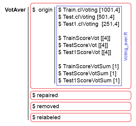
Fig. 10. The data structure of VotAver.
The figure below provides a simplified scheme of all calculations: it shows the stages, the used scripts and data structures.
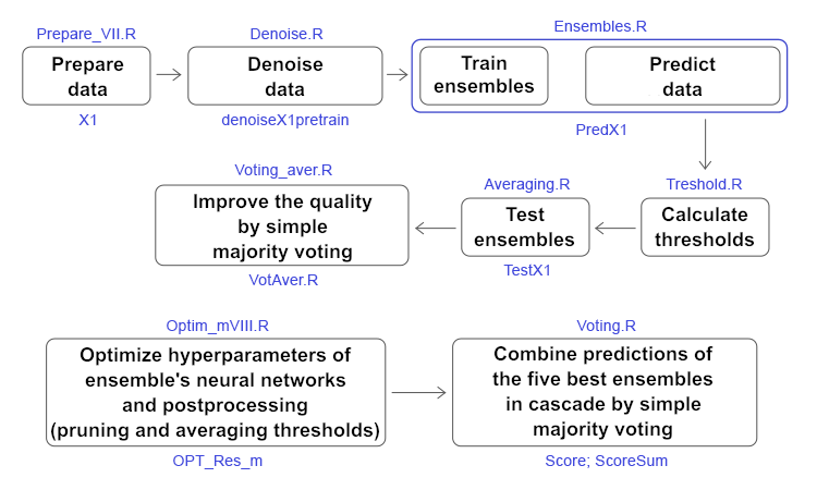
Fig. 11. Structure and sequence of the main calculations in the article.
8. Analyzing experimental results
We have processed the noise samples from the initial data sets in the pretrain subsets (!) in three ways:
- reallocated the "erroneously" labeled data without changing the number of classes (repaired);
- removed the "noise" samples from the subset (removed);
- isolated the "noise" samples in a separate class (relabeled).
Four groups of data (origin, repaired, removed, relabeled) were obtained in the denoiseX1pretrain structure. Use them to train the ensemble consisting of 500 ELM neural network classifiers. Obtain four ensembles. Calculate the continuous predictions of three subsets Х1$train/test/test1 using these 4 ensembles and collect them into the predX1 structure.
Then calculate 4 types of thresholds for continuous predictions of each of the 500 neural networks of each ensemble on the InputTrain subset (!). Using these thresholds, convert the continuous predictions into class labels (0, 1). Calculate the metrics (mean(F1)) for each neural network of the ensembles and collect them in the structure testX1$$(InputTrainScore|InputTestScore|InputTest1Score). Visualization of the metrics' distribution in 4 data groups and 3 subsets shows:
- first, the metrics on the first test subset are higher than on InputTrainS in all groups;
- second, the metrics are visually higher in the repaired and removed groups than in two others.
Now select the 7 best neural networks with the largest values of mean(F1) in each ensemble and average their continuous predictions. Add their values to the structure testX1$$(TrainYpred|TestYpred|Test1Ypred). Calculate the thresholds th_aver on the subset TrainYpred, determine the metrics of all averaged continuous predictions and add them to the structure testX1$$(TrainScore|TestScore|Test1Score). Now they can be analyzed.
With different combination of the pruning and averaging thresholds in different data groups, we obtain metrics in the range of 0.75 — 0.77. The best result has been obtained in the removed group with the "noise" samples removed.
Optimization of the neural networks' hyperparameters provides a stable increase in metrics of 0.77+ in all groups.
Optimization of the neural networks' hyperparameters and postprocessing (pruning and averaging) thresholds provides a stably high result of about 0.78+ in all groups with the processed "noise" samples.
Create a superensemble from several ensembles with the optimal hyperparameters, take the predictions of these ensembles and combine them by a simple majority voting in each data group. As a result, obtain the metrics in groups repaired and removed in the range of 0.82+. Combining these predictions of the superensembles by simple majority voting as well, obtain the final metric value of 0.836. Thus, combining the predictions in cascade by simple majority voting gives an improvement in quality of 6-7%.
Verify this statement on the averaged predictions of the ensemble received early. After repeating the calculations and conversions in the groups, receive metrics of 0.8+ in the removed group of the Test subset. Continuing the combination in cascade, receive metrics with values of 0,8+ in the Test subset in all data groups.
It can be concluded that combining the ensemble predictions in cascade by simple voting improves the classification quality indeed.
Conclusion
In this article, three methods for improving the quality of bagging ensembles have been considered, as well as optimization of hyperparameters of the ensemble's neural networks and postprocessing. Based on the results of the experiments, the following conclusions can be drawn:
- processing the noise samples using the repaired and removed methods significantly improves the classification quality of ensembles;
- selecting the threshold type for pruning and averaging, as well as their combination significantly affect the classification quality;
- combining several ensembles into a superensemble with their predictions combined in cascade by simple majority voting gives the greatest increase in the classification quality;
- optimizing the hyperparameters of ensembles' neural networks and post processing slightly improves the classification quality scores. It is advisable to perform the first optimization on new data, and them repeat it periodically when the quality decreases. Periodicity is determined experimentally.
Attachments
GitHub/PartVIII contains the following files:
- Importar.R — package import functions.
- Library.R — required libraries.
- FunPrepareData_VII.R — functions for preparing initial data.
- FunStacking_VIII.R — functions for creating and testing the ensemble.
- Prepare_VIII.R — functions and scripts for preparing the initial data for trainable combiners.
- Denoise.R — scripts for processing noise samples.
- Ensemles.R — scripts for creating ensembles.
- Threshold.R — scripts for determining thresholds.
- Test.R — scripts for testing ensembles.
- Averaging.R — scripts for averaging continuous outputs of ensembles.
- Voting_aver.R — combining averaged outputs in cascade by simple majority voting.
- Optim_VIII.R — scripts for optimization the hyperparameters of neural networks.
- Optim_mVIII.R — scripts for optimization the hyperparameters of neural networks and postprocessing.
- Voting.R — combining outputs of the superensemble in cascade by simple majority voting.
- SessionInfo_VII.txt — list of packages used in the article scripts.