Data Science and Machine Learning (Part 11): Naïve Bayes, Probability theory in Trading
Omega J Msigwa | 3 March, 2023
Fourth Law of Thermodynamics: If the probability of success is not almost one, then it is damn near zero.
David J. Rose
Introduction
Naïve Bayes classifier is a probabilistic algorithm used in machine learning for classification tasks. It is based on Bayes' theorem, which calculates the probability of a hypothesis given the available evidence. This probabilistic classifier is a simple yet effective algorithm in various situations. It assumes that the features used for classification are independent of each other. For example: If you want this model to classify humans(male and female) given height, foot size, weight, and shoulder length, this model treats all these variables as independent of each other, In this case, it doesn't even think that foot size and height are related for a human.
Since this model doesn't bother understanding the patterns between the independent variables, I think we should give it a shot by trying to use it to make informed trading decisions. I believe in the trading space nobody fully understands the patterns anyway so, let's see how the Naïve Bayes performs.
Without further ado, let's call the model instance and use it right away. We'll discuss to see what this model is made up of later on.
Preparing Training Data
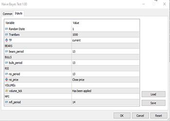
For this example, I chose 5 Indicators, most of them oscillators and volumes as I think they make good classification variables also they have a finite amount which makes them good for normal distribution which is one of the ideas at the core of this algorithm, You are not restricted to these indicators though, so feel free to explore various indicators and data you would prefer.
First things first:
matrix Matrix(TrainBars, 6);
int handles[5];

double buffer[];
//+------------------------------------------------------------------+
//| Expert initialization function                                   |
//+------------------------------------------------------------------+
int OnInit()
  {
//--- Preparing Data
   handles[0] = iBearsPower(Symbol(),TF, bears_period);
   handles[1] = iBullsPower(Symbol(),TF, bulls_period);
   handles[2] = iRSI(Symbol(),TF,rsi_period, rsi_price);
   handles[3] = iVolumes(Symbol(),TF,VOLUME_TICK);
   handles[4] = iMFI(Symbol(),TF,mfi_period,VOLUME_TICK );

//---
   vector col_v;
   for (ulong i=0; i<5; i++) //Independent vars
     {
       CopyBuffer(handles[i],0,0,TrainBars, buffer);
       col_v = matrix_utils.ArrayToVector(buffer);

       Matrix.Col(col_v, i);
     }
//-- Target var
   vector open, close;
   col_v.Resize(TrainBars);

   close.CopyRates(Symbol(),TF, COPY_RATES_CLOSE,0,TrainBars);
   open.CopyRates(Symbol(),TF, COPY_RATES_OPEN,0,TrainBars);

   for (int i=0; i<TrainBars; i++)
      {
         if (close[i] > open[i]) //price went up
            col_v[i] = 1;
         else
            col_v[i] = 0;
      }

   Matrix.Col(col_v, 5); //Adding independent variable to the last column of matrix
//---
The variables TF, bears_period etc. Are input defined variables that are found on top of the above code:
Since this is supervised learning, I had to make up the target variable, the logic is simple. If the close price was above the opening price the target variable is set to class 1 otherwise the class is 0. This is how the target variable was set. Below is an overview of how the dataset matrix looks like:
CS      0       13:21:15.457    Naive Bayes Test (EURUSD,H1)    "Bears"           "Bulls"        "Rsi"      "Volumes" "MFI"     "Target Var"
CS      0       13:21:15.457    Naive Bayes Test (EURUSD,H1)    [-3.753148029472797e-06,0.008786246851970603,67.65238281791684,13489,55.24611392389958,0]
CS      0       13:21:15.457    Naive Bayes Test (EURUSD,H1)    [-0.002513216984025402,0.005616783015974569,50.29835423473968,12226,49.47293811405203,1]
CS      0       13:21:15.457    Naive Bayes Test (EURUSD,H1)    [-0.001829900272021678,0.0009700997279782353,47.33479153312328,7192,46.84320886771249,1]
CS      0       13:21:15.457    Naive Bayes Test (EURUSD,H1)    [-0.004718485947447171,-0.0001584859474472733,39.04848493977027,6267,44.61564654651691,1]
CS      0       13:21:15.457    Naive Bayes Test (EURUSD,H1)    [-0.004517273669240485,-0.001367273669240276,45.4127802340401,3867,47.8438816641815,0]
I then decided to visualize the data in Distribution Plots to see if they follow the Probability Distribution:


There is an entire article for those wanting to understand different kinds of probability distribution linked here.
If you take a closer look at the correlation coefficient matrix of all the independent variables:
   string header[5] = {"Bears","Bulls","Rsi","Volumes","MFI"};

   matrix vars_matrix = Matrix; //Independent variables only
   matrix_utils.RemoveCol(vars_matrix, 5); //remove target variable

   ArrayPrint(header);
   Print(vars_matrix.CorrCoef(false));
Output:
CS      0       13:21:15.481    Naive Bayes Test (EURUSD,H1)    "Bears"   "Bulls"   "Rsi"     "Volumes" "MFI"
CS      0       13:21:15.481    Naive Bayes Test (EURUSD,H1)    [[1,0.7784600081627714,0.8201955846987788,-0.2874457184671095,0.6211980865273238]
CS      0       13:21:15.481    Naive Bayes Test (EURUSD,H1)     [0.7784600081627714,1,0.8257210032763984,0.2650418244580489,0.6554288778228361]
CS      0       13:21:15.481    Naive Bayes Test (EURUSD,H1)     [0.8201955846987788,0.8257210032763984,1,-0.01205084357067248,0.7578863565293196]
CS      0       13:21:15.481    Naive Bayes Test (EURUSD,H1)     [-0.2874457184671095,0.2650418244580489,-0.01205084357067248,1,0.0531475992791923]
CS      0       13:21:15.481    Naive Bayes Test (EURUSD,H1)     [0.6211980865273238,0.6554288778228361,0.7578863565293196,0.0531475992791923,1]]
You will notice that except for volumes correlation to the rest, all the variables are strongly correlated to each other, some a coincidence for example RSI vs both Bulls and Bears with a correlation of about 82%. Volumes and MFI have common stuff they are both made up of which is volumes so they have a reason to be 62% correlated. Since the Gaussian Naïve Bayes doesn't care about any of that stuff let's move on but I thought it is a good idea to check and analyze the variables.
Training the Model
Training the Gaussian Naïve Bayes is simple and takes a very short time. Let's first see how to properly do it:
     Print("\n---> Training the Model\n");

     matrix x_train, x_test;
     vector y_train, y_test;

     matrix_utils.TrainTestSplitMatrices(Matrix,x_train,y_train,x_test,y_test,0.7,rand_state);

//--- Train
     gaussian_naive = new CGaussianNaiveBayes(x_train,y_train);  //Initializing and Training the model
     vector train_pred = gaussian_naive.GaussianNaiveBayes(x_train); //making predictions on trained data
     vector c= gaussian_naive.classes; //Classes in a dataset that was detected by mode
     metrics.confusion_matrix(y_train,train_pred,c);  //analyzing the predictions in confusion matrix
//---
The function TrainTestSplitMatrices splits the data into x training and x testing matrices and their respective target vectors. Just like train_test_split in sklearn python. The function at it core goes like this:
void CMatrixutils::TrainTestSplitMatrices(matrix &matrix_,matrix &x_train,vector &y_train,matrix &x_test, vector &y_test,double train_size=0.7,int random_state=-1)
By default, 70 percent of the data will be split into the training data and the rest will be kept as the testing dataset, Read for more information about this splitting.
What a lot of folks found confusing in this function is the random_state, people often choose random_state=42 in the Python ML community, even though any number will be fine as this number is just for ensuring the randomized/shuffled matrix is generated the same each time to make it easier to debug since it sets the Random seed for Generating random numbers for shuffling the rows in a matrix.
You may notice that the output matrices obtained by this function are not in the default order they were. There are several discussions about choosing this 42 number.
Below is the output of this block of code:
CS      0       14:33:04.001    Naive Bayes Test (EURUSD,H1)    ---> Training the Model
CS      0       14:33:04.001    Naive Bayes Test (EURUSD,H1)
CS      0       14:33:04.002    Naive Bayes Test (EURUSD,H1)    ---> GROUPS [0,1]
CS      0       14:33:04.002    Naive Bayes Test (EURUSD,H1)
CS      0       14:33:04.002    Naive Bayes Test (EURUSD,H1)    ---> Prior_proba [0.5457142857142857,0.4542857142857143] Evidence [382,318]

CS      0       14:33:04.294    Naive Bayes Test (EURUSD,H1)    Confusion Matrix
CS      0       14:33:04.294    Naive Bayes Test (EURUSD,H1)    [[236,146]
CS      0       14:33:04.294    Naive Bayes Test (EURUSD,H1)     [145,173]]
CS      0       14:33:04.294    Naive Bayes Test (EURUSD,H1)
CS      0       14:33:04.294    Naive Bayes Test (EURUSD,H1)    Classification Report
CS      0       14:33:04.294    Naive Bayes Test (EURUSD,H1)
CS      0       14:33:04.294    Naive Bayes Test (EURUSD,H1)    _    Precision  Recall  Specificity  F1 score  Support
CS      0       14:33:04.294    Naive Bayes Test (EURUSD,H1)    0.0    0.62     0.62     0.54       0.62     382.0
CS      0       14:33:04.294    Naive Bayes Test (EURUSD,H1)    1.0    0.54     0.54     0.62       0.54     318.0
CS      0       14:33:04.294    Naive Bayes Test (EURUSD,H1)
CS      0       14:33:04.294    Naive Bayes Test (EURUSD,H1)    Accuracy                                   0.58
CS      0       14:33:04.294    Naive Bayes Test (EURUSD,H1)    Average   0.58    0.58    0.58      0.58    700.0
CS      0       14:33:04.294    Naive Bayes Test (EURUSD,H1)    W Avg     0.58    0.58    0.58      0.58    700.0
CS      0       14:33:04.294    Naive Bayes Test (EURUSD,H1)
The trained model is 58% Accurate according to the confusion matrix classification report. There is a lot you can understand from that report such as the precision which tells how accurately each class was classified read more. Basically, Class 0 seemed to be classified better than class 1, which makes sense because the model has predicted it more than the other class 1 not to mention the Prior Probability, which is the primary probability or the probability at first glance in the dataset. In this dataset the prior probabilities are:
Prior_proba [0.5457142857142857,0.4542857142857143] Evidence [382,318]. This prior probability is calculated as:
Prior Proba = Evidence/ Total number of events/outcomes
In this case Prior Proba [382/700, 318/700]. Remember 700 is the training dataset size we have after splitting 70% of 1000 data to train data?
The Gaussian Naïve Bayes model first looks at the probabilities of the classes to occur in a dataset and then uses those to guess what might happen in the future, this is calculated based off evidence. The class with higher evidence leading to higher probability than the other will be favored by the algorithm when training and testing. It makes sense right? This is one of the disadvantages of this algorithm because when a class is not present in the training data the model assumes that, that class doesn't happen so it gives it the probability of zero, meaning it won't be predicted in the testing dataset or anytime in the future.
Testing the model
Testing the model is easy too. All you need is to plug the new data into the function GaussianNaiveBayes which has parameters of the trained model already to this point.
//--- Test
     Print("\n---> Testing the model\n");
     vector test_pred = gaussian_naive.GaussianNaiveBayes(x_test); //giving the model test data to predict and obtain predictions to a vector
     metrics.confusion_matrix(y_test,test_pred, c); //analyzing the tested model
Outputs:
CS      0       14:33:04.294    Naive Bayes Test (EURUSD,H1)    ---> Testing the model
CS      0       14:33:04.294    Naive Bayes Test (EURUSD,H1)
CS      0       14:33:04.418    Naive Bayes Test (EURUSD,H1)    Confusion Matrix
CS      0       14:33:04.418    Naive Bayes Test (EURUSD,H1)    [[96,54]
CS      0       14:33:04.418    Naive Bayes Test (EURUSD,H1)     [65,85]]
CS      0       14:33:04.418    Naive Bayes Test (EURUSD,H1)
CS      0       14:33:04.418    Naive Bayes Test (EURUSD,H1)    Classification Report
CS      0       14:33:04.418    Naive Bayes Test (EURUSD,H1)
CS      0       14:33:04.418    Naive Bayes Test (EURUSD,H1)    _    Precision  Recall  Specificity  F1 score  Support
CS      0       14:33:04.418    Naive Bayes Test (EURUSD,H1)    0.0    0.60     0.64     0.57       0.62     150.0
CS      0       14:33:04.418    Naive Bayes Test (EURUSD,H1)    1.0    0.61     0.57     0.64       0.59     150.0
CS      0       14:33:04.418    Naive Bayes Test (EURUSD,H1)
CS      0       14:33:04.418    Naive Bayes Test (EURUSD,H1)    Accuracy                                   0.60
CS      0       14:33:04.418    Naive Bayes Test (EURUSD,H1)    Average   0.60    0.60    0.60      0.60    300.0
CS      0       14:33:04.418    Naive Bayes Test (EURUSD,H1)    W Avg     0.60    0.60    0.60      0.60    300.0
Great, so the model has performed slightly better on the testing data set, giving 60% accuracy 2% increase from the training data accuracy so that's some good news.
The Gaussian Naïve Bayes Model in the Strategy Tester
Using machine learning models on the Strategy Tester often do not perform well, not because they couldn't make predictions but because we usually look at the profits graph on the strategy tester. A machine learning model being able to guess where the market heads next doesn't necessarily mean you will make money out of it, especially with the simple logic I used to collect and prepare our dataset. See the datasets were collected on each bar using the TF that were given in the input which is PERIOD_H1 (One hour).
   close.CopyRates(Symbol(),TF, COPY_RATES_CLOSE,0,TrainBars);
   open.CopyRates(Symbol(),TF, COPY_RATES_OPEN,0,TrainBars);
I gathered 1000 bars from a one-hour timeframe, read their indicator values as independent variables. I then created the target variables by looking if the candle was bullish our EA sets the class 1 otherwise sets the class 0. So when I created the function to trade I took this into account. Since our model will be predicting the next candle then I was opening trades on each new candle and close the previous ones. Basically, letting our EA trade on every signal in every bar.
//+------------------------------------------------------------------+
//| Expert tick function                                             |
//+------------------------------------------------------------------+
void OnTick()
  {
   if (!train_state)
      TrainTest();

    train_state = true;

//---
   vector v_inputs(5); //5 independent variables
   double buff[1];  //current indicator value

   for (ulong i=0; i<5; i++) //Independent vars
     {
       CopyBuffer(handles[i],0,0,1, buff);

       v_inputs[i] = buff[0];
     }

//---
   MqlTick ticks;
   SymbolInfoTick(Symbol(), ticks);

   int signal = -1;
   double min_volume = SymbolInfoDouble(Symbol(), SYMBOL_VOLUME_MIN);

   if (isNewBar())
     {
       signal = gaussian_naive.GaussianNaiveBayes(v_inputs);
       Comment("SIGNAL ",signal);
       CloseAll();

        if (signal == 1)
          {
            if (!PosExist())
              m_trade.Buy(min_volume, Symbol(), ticks.ask, 0 , 0,"Naive Buy");
          }
        else if (signal == 0)
          {
            if (!PosExist())
              m_trade.Sell(min_volume, Symbol(), ticks.bid, 0 , 0,"Naive Sell");
          }
     }
  }
To make this function work in both live trading and Strategy Tester too, I had to change the logic a bit, Indicator CopyBuffer() and training are now inside the TrainTest() function. This function is run once on the On Tick function, you can make it run often to train the model very often but I leave that for you to exercise.
Since the Init function is not the function suitable for all those copy buffer and copy rates methods (They return zero values on Strategy Tester when used this way), everything is now moved to the Function TrainTest().
int OnInit()
  {
   handles[0] = iBearsPower(Symbol(),TF, bears_period);
   handles[1] = iBullsPower(Symbol(),TF, bulls_period);
   handles[2] = iRSI(Symbol(),TF,rsi_period, rsi_price);
   handles[3] = iVolumes(Symbol(),TF,VOLUME_TICK);
   handles[4] = iMFI(Symbol(),TF,mfi_period,VOLUME_TICK );

//---

   m_trade.SetExpertMagicNumber(MAGIC_NUMBER);
   m_trade.SetTypeFillingBySymbol(Symbol());
   m_trade.SetMarginMode();
   m_trade.SetDeviationInPoints(slippage);

   return(INIT_SUCCEEDED);
  }
Single Test: 1 hour Timeframe
I ran a test for two months from January 1st 2023, to February 14th 2023 (yesterday):
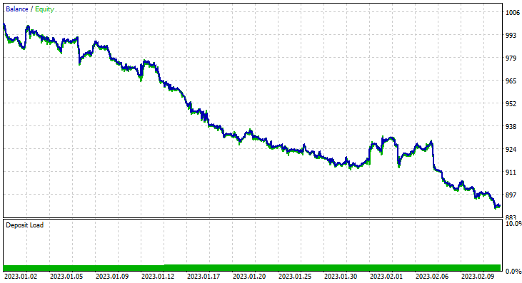
I decided to run a test for such a short period (2 Months) because 1000 one-hour bars, is not such a long training period Nearly 41 days so, the training period is a short time and the testing too. Since the TrainTest() function was also run on the Tester. The candles that the model was trained on are 700 bars.
What went wrong?
The model did make the first Impression on the strategy tester by giving an impressive 60% accuracy on the training data.
CS      0       08:30:13.816    Tester  initial deposit 1000.00 USD, leverage 1:100
CS      0       08:30:13.818    Tester  successfully initialized
CS      0       08:30:13.818    Network 80 Kb of total initialization data received
CS      0       08:30:13.819    Tester  Intel Core i5  660 @ 3.33GHz, 6007 MB
CS      0       08:30:13.900    Symbols EURUSD: symbol to be synchronized
CS      0       08:30:13.901    Symbols EURUSD: symbol synchronized, 3720 bytes of symbol info received
CS      0       08:30:13.901    History EURUSD: history synchronization started
....
....
....
CS      0       08:30:14.086    Naive Bayes Test (EURUSD,H1)    2023.01.02 01:00:00   ---> Training the Model
CS      0       08:30:14.086    Naive Bayes Test (EURUSD,H1)    2023.01.02 01:00:00
CS      0       08:30:14.086    Naive Bayes Test (EURUSD,H1)    2023.01.02 01:00:00   ---> GROUPS [0,1]
CS      0       08:30:14.086    Naive Bayes Test (EURUSD,H1)    2023.01.02 01:00:00
CS      0       08:30:14.086    Naive Bayes Test (EURUSD,H1)    2023.01.02 01:00:00   ---> Prior_proba [0.4728571428571429,0.5271428571428571] Evidence [331,369]
CS      0       08:30:14.377    Naive Bayes Test (EURUSD,H1)    2023.01.02 01:00:00   Confusion Matrix
CS      0       08:30:14.378    Naive Bayes Test (EURUSD,H1)    2023.01.02 01:00:00   [[200,131]
CS      0       08:30:14.378    Naive Bayes Test (EURUSD,H1)    2023.01.02 01:00:00    [150,219]]
CS      0       08:30:14.378    Naive Bayes Test (EURUSD,H1)    2023.01.02 01:00:00
CS      0       08:30:14.378    Naive Bayes Test (EURUSD,H1)    2023.01.02 01:00:00   Classification Report
CS      0       08:30:14.378    Naive Bayes Test (EURUSD,H1)    2023.01.02 01:00:00
CS      0       08:30:14.378    Naive Bayes Test (EURUSD,H1)    2023.01.02 01:00:00   _    Precision  Recall  Specificity  F1 score  Support
CS      0       08:30:14.378    Naive Bayes Test (EURUSD,H1)    2023.01.02 01:00:00   0.0    0.57     0.60     0.59       0.59     331.0
CS      0       08:30:14.378    Naive Bayes Test (EURUSD,H1)    2023.01.02 01:00:00   1.0    0.63     0.59     0.60       0.61     369.0
CS      0       08:30:14.378    Naive Bayes Test (EURUSD,H1)    2023.01.02 01:00:00
CS      0       08:30:14.378    Naive Bayes Test (EURUSD,H1)    2023.01.02 01:00:00   Accuracy                                   0.60
CS      0       08:30:14.378    Naive Bayes Test (EURUSD,H1)    2023.01.02 01:00:00   Average   0.60    0.60    0.60      0.60    700.0
CS      0       08:30:14.378    Naive Bayes Test (EURUSD,H1)    2023.01.02 01:00:00   W Avg     0.60    0.60    0.60      0.60    700.0
However, it couldn't make profitable trades of that promised accuracy or anywhere near that. Below are my observations:
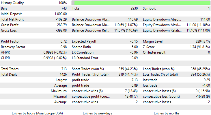
- The Logic is somehow blind, It trades quantity for quality. 713 Trades over the course of two months. C'mon, that's a lot of trades. This needs to be changed to its opposite. We need to train this model on a higher timeframe and trade on higher timeframes resulting in few quality trades.
- Training Bars have to be reduced for this test, I want to train the model on recent data.
To achieve these I ran optimization on 6H Timeframe, and came out with Train Bars = 80, TF = 12 hours, I then ran a test for (2 months using the new parameters). Check out all parameters in the *set file linked at the end of this article.
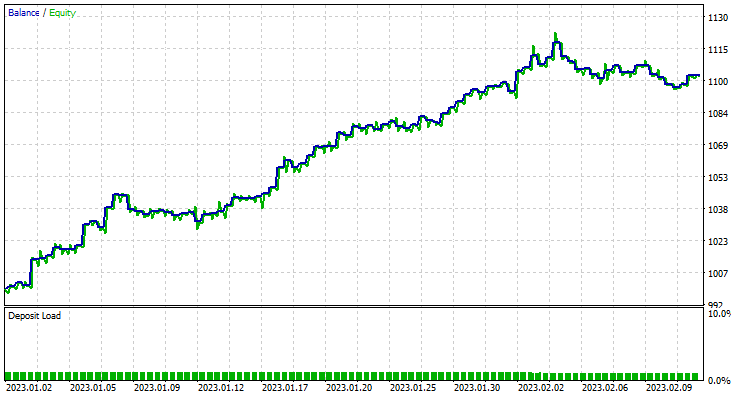
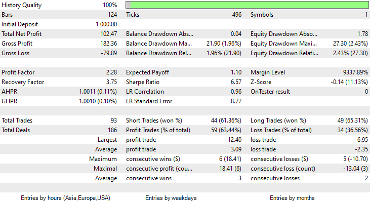
This time the training accuracy of the Gaussian Naïve Bayes model was 58% percent.
93 Trades over the course of 2 Months, that's what I call healthy trading activity, averaging 2.3 trades a day. This time the Gaussian Naïve Bayes EA made 63% trades profitable not to mention about a 10% profit.
Now that you have seen how you can use the Gaussian Naïve Bayes model to make informed trading decisions, let's see what makes it tick.
Naïve Bayes Theory
Not to be confused with Gaussian Naïve Bayes.
The algorithm is called
- Naïve because it assumes that the variables/features are independent, which is rarely the case
-
Bayes because it is based on the Bayes theorem
The formula for the Bayes theorem is given below:

Where;
P(A|B) = Posterior probability or Probability of hypothesis A on the observed event B
P(B|A) = Likelihood probability : Probability of the evidence given that the probability of the hypothesis is true. In simple words Probability of B given A is true
P(A) = Is a prior probability of A or probability of the hypothesis before observing the evidence
P(B) = Is marginal probability : Probability of the evidence
These terminologies in the formula might seem confusing at first. They will become clear in action so stick with me.
Working with the Classifier
Let's take a look at a simple example on the Weather dataset. Let's focus on the single first column Outlook, Once that is understood adding other columns as independent variables is just the exact-same process.
| Outlook | Play Tennis |
|---|---|
| Sunny | No |
| Sunny | No |
| Overcast | Yes |
| Rain | Yes |
| Rain | Yes |
| Rain | No |
| Overcast | Yes |
| Sunny | No |
| Sunny | Yes |
| Rain | Yes |
| Sunny | Yes |
| Overcast | Yes |
| Overcast | Yes |
| Rain | No |
Now, Let us do the same thing in MetaEditor:
void OnStart()
  {
//---
   matrix Matrix = matrix_utils.ReadCsvEncode("weather dataset.csv");

   int cols[3] = {1,2,3};

   matrix_utils.RemoveMultCols(Matrix, cols); //removing Temperature Humidity and Wind
   ArrayRemove(matrix_utils.csv_header,1,3); //removing column headers

   ArrayPrint(matrix_utils.csv_header);
   Print(Matrix);

   matrix x_matrix; vector y_vector;

   matrix_utils.XandYSplitMatrices(Matrix, x_matrix, y_vector);

  }
Keep in mind that the Naïve Bayes is for discrete/non-continuous variables only. Not to be confused with the Gaussian Naïve Bayes we have seen in action above, which can deal with continuous variables, the case is different for this Naïve Bayes model, That's why in this example I decided to use this dataset that contains the discrete values that have been encoded from string values. Below is the output of the above operation
CS      0       12:59:37.386    Naive Bayes theory script (EURUSD,H1)   "Outlook" "Play"
CS      0       12:59:37.386    Naive Bayes theory script (EURUSD,H1)   [[0,0]
CS      0       12:59:37.386    Naive Bayes theory script (EURUSD,H1)    [0,0]
CS      0       12:59:37.386    Naive Bayes theory script (EURUSD,H1)    [1,1]
CS      0       12:59:37.386    Naive Bayes theory script (EURUSD,H1)    [2,1]
CS      0       12:59:37.386    Naive Bayes theory script (EURUSD,H1)    [2,1]
CS      0       12:59:37.386    Naive Bayes theory script (EURUSD,H1)    [2,0]
CS      0       12:59:37.386    Naive Bayes theory script (EURUSD,H1)    [1,1]
CS      0       12:59:37.386    Naive Bayes theory script (EURUSD,H1)    [0,0]
CS      0       12:59:37.386    Naive Bayes theory script (EURUSD,H1)    [0,1]
CS      0       12:59:37.386    Naive Bayes theory script (EURUSD,H1)    [2,1]
CS      0       12:59:37.386    Naive Bayes theory script (EURUSD,H1)    [0,1]
CS      0       12:59:37.386    Naive Bayes theory script (EURUSD,H1)    [1,1]
CS      0       12:59:37.386    Naive Bayes theory script (EURUSD,H1)    [1,1]
CS      0       12:59:37.386    Naive Bayes theory script (EURUSD,H1)    [2,0]]
That being said, let's find the prior probability in our Naïve Bayes class constructor:
CNaiveBayes::CNaiveBayes(matrix &x_matrix, vector &y_vector)
 {
   XMatrix.Copy(x_matrix);
   YVector.Copy(y_vector);

   classes = matrix_utils.Classes(YVector);

   c_evidence.Resize((ulong)classes.Size());

   n = YVector.Size();

   if (n==0) { Print("--> n == 0 | Naive Bayes class failed"); return; }

//---

   vector v = {};
   for (ulong i=0; i<c_evidence.Size(); i++)
       {
         v = matrix_utils.Search(YVector,(int)classes[i]);

         c_evidence[i] = (int)v.Size();
       }

//---

   c_prior_proba.Resize(classes.Size());

   for (ulong i=0; i<classes.Size(); i++)
      c_prior_proba[i] = c_evidence[i]/(double)n;


   #ifdef DEBUG_MODE
      Print("---> GROUPS ",classes);
      Print("Prior Class Proba ",c_prior_proba,"\nEvidence ",c_evidence);
   #endif

 }
Outputs:
CS      0       12:59:37.386    Naive Bayes theory script (EURUSD,H1)   ---> GROUPS [0,1]
CS      0       12:59:37.386    Naive Bayes theory script (EURUSD,H1)   Prior Class Proba [0.3571428571428572,0.6428571428571429]
CS      0       12:59:37.386    Naive Bayes theory script (EURUSD,H1)   Evidence [5,9]
The prior probability of [No, Yes] is approximately [0.36, 0.64]
Now, let's say you want to know the probability of a person playing Tennis on a Sunny day, here is what you will do;
P(Yes | Sunny) = P(Sunny | Yes) * P(Yes) / P(Sunny)
More details in simple English:
Probability of someone playing on a sunny day = how many times in terms of probability it was sunny and some fool played Tennis * how many times in probability terms, People played tennis / how many times in probability terms it was a sunny day in general.
P(Sunny | Yes) = 2/9
P(Yes) = 0.64
P(Sunny) = 5/14 = 0.357
so finally the P(Yes | Sunny) = 0.333 x 0.64 / 0.357 = 0.4
What about the Probability of (No| Sunny): You can calculate it by taking 1- Probability of yes = 1 - 0.5972 = 0.4027 As a shortcut but let's see about it too;
P(No|Sunny) = (3/5) x 0.36 / (0.357) = 0.6
Below is the code to do it:
vector CNaiveBayes::calcProba(vector &v_features)
 {
    vector proba_v(classes.Size()); //vector to return

    if (v_features.Size() != XMatrix.Cols())
      {
         printf("FATAL | Can't calculate probability,  features columns size = %d is not equal to XMatrix columns =%d",v_features.Size(),XMatrix.Cols());
         return proba_v;
      }

//---

    vector v = {};

    for (ulong c=0; c<classes.Size(); c++)
      {
        double proba = 1;
          for (ulong i=0; i<XMatrix.Cols(); i++)
            {
                v = XMatrix.Col(i);

                int count =0;
                for (ulong j=0; j<v.Size(); j++)
                  {
                     if (v_features[i] == v[j] && classes[c] == YVector[j])
                        count++;
                  }

                proba *= count==0 ? 1 : count/(double)c_evidence[c]; //do not calculate if there isn't enough evidence'
            }

        proba_v[c] = proba*c_prior_proba[c];
     }

    return proba_v;
 }
The probability vector provided by this function for sunny are:
2023.02.15 16:34:21.519 Naive Bayes theory script (EURUSD,H1) Probabilities [0.6,0.4]
Exactly what we expected, but make no mistake this function doesn't give us the probabilities. Let me explain, when there are two classes only in the dataset you are trying to predict in that scenario the outcome is a probability but other wise, the outputs of this function needs to be validated into probability terms, to achieve that is simple:
Take the sum of the vector that came out of this function, then divide each element to the total sum, the remaining vector will be the real probability values that when summed up will be equal to one.
probability_v = v[i]/probability_v.Sum()
This small process is performed inside the function NaiveBayes() which predicts the outcome class or the class with the higher probability of all:
int CNaiveBayes::NaiveBayes(vector &x_vector)
 {
   vector v = calcProba(x_vector);

   double sum = v.Sum();

   for (ulong i=0; i<v.Size(); i++) //converting the values into probabilities
      v[i] = NormalizeDouble(v[i]/sum,2);

   vector p = v;

   #ifdef   DEBUG_MODE
      Print("Probabilities ",p);
   #endif

   return((int)classes[p.ArgMax()]);
 }
Well that's it. The Naïve Bayes is a simple algorithm, Now let's shift the focus to the Gaussian Naïve Bayes which is the one we used early in this article.
Gaussian Naïve Bayes
The gaussian naïve Bayes assumes that features follow a normal distribution, this means if predictors take on continuous variables instead of discrete then it assumes that these values are sampled from the Gaussian Distribution.
A recap on Normal Distribution
The normal distribution is a continuous probability distribution that is symmetrical around its mean, most of the observations cluster around the central peak, and the probabilities for values further away from the mean taper off equally in both directions. Extreme values in both tails of the distribution are similarly unlikely.

This bell-shaped probability curve is so powerful, it is one among the useful statistical analysis tools. It shows that there is an approximate 34% probability of finding something one standard deviation away from the mean and 34% of finding something on the other side of the bell curve. Meaning there is about 68% chance of finding a value that lies one standard away from the mean on both sides combined. Those who skipped mathematics class should continue reading.
From this normal distribution/Gaussian distribution we want to find the probability density. It is calculated using the formula below.
![]()
Where:
μ = Mean
𝜎 = Standard Deviation
x = input value
Ok, since the Gaussian Naïve Bayes depends on this let's code for it.
class CNormDistribution
  {

public:

   double m_mean; //Assign the value of the mean
   double m_std;  //Assign the value of Variance

                     CNormDistribution(void);
                    ~CNormDistribution(void);

                     double PDF(double x); //Probability density function
  };
//+------------------------------------------------------------------+
//|                                                                  |
//+------------------------------------------------------------------+

CNormDistribution::CNormDistribution(void)
 {

 }

//+------------------------------------------------------------------+
//|                                                                  |
//+------------------------------------------------------------------+

CNormDistribution::~CNormDistribution(void)
 {
   ZeroMemory(m_mean);
   ZeroMemory(m_std);
 }

//+------------------------------------------------------------------+
//|                                                                  |
//+------------------------------------------------------------------+

double CNormDistribution::PDF(double x)
 {
   double nurm = MathPow((x - m_mean),2)/(2*MathPow(m_std,2));
   nurm = exp(-nurm);

   double denorm = 1.0/(MathSqrt(2*M_PI*MathPow(m_std,2)));

  return(nurm*denorm);
 }
Creating the Gaussian Naïve Bayes Model
The class constructor of the Gaussian Naïve Bayes looks similar to that of the Naïve Bayes. No need to show and explain the constructor code here. Below is our main function that's responsible for calculating the probability.
vector CGaussianNaiveBayes::calcProba(vector &v_features)
 {
    vector proba_v(classes.Size()); //vector to return

    if (v_features.Size() != XMatrix.Cols())
      {
         printf("FATAL | Can't calculate probability, features columns size = %d is not equal to XMatrix columns =%d",v_features.Size(),XMatrix.Cols());
         return proba_v;
      }

//---
    vector v = {};

    for (ulong c=0; c<classes.Size(); c++)
      {
        double proba = 1;
          for (ulong i=0; i<XMatrix.Cols(); i++)
            {
                v = XMatrix.Col(i);
                int count =0;
                vector calc_v = {};

                for (ulong j=0; j<v.Size(); j++)
                  {
                     if (classes[c] == YVector[j])
                       {
                         count++;
                         calc_v.Resize(count);

                         calc_v[count-1] = v[j];
                       }
                  }

                norm_distribution.m_mean = calc_v.Mean(); //Assign these to Gaussian Normal distribution
                norm_distribution.m_std = calc_v.Std();

                #ifdef DEBUG_MODE
                  printf("mean %.5f std %.5f ",norm_distribution.m_mean,norm_distribution.m_std);
                #endif

                proba *= count==0 ? 1 : norm_distribution.PDF(v_features[i]); //do not calculate if there isn't enought evidence'
            }

        proba_v[c] = proba*c_prior_proba[c]; //Turning the probability density into probability

        #ifdef DEBUG_MODE
         Print(">> Proba ",proba," prior proba ",c_prior_proba);
        #endif
     }

    return proba_v;
 }
Let's see how this model performs in action.
Using the Gender dataset.
| Height(ft) | Weight(lbs) | Foot Size(inches | Person(0 male, 1 female) |
|---|---|---|---|
| 6 | 180 | 12 | 0 |
| 5.92 | 190 | 11 | 0 |
| 5.58 | 170 | 12 | 0 |
| 5.92 | 165 | 10 | 0 |
| 5 | 100 | 6 | 1 |
| 5.5 | 150 | 8 | 1 |
| 5.42 | 130 | 7 | 1 |
| 5.75 | 150 | 9 | 1 |
//--- Gaussian naive bayes
   Matrix = matrix_utils.ReadCsv("gender dataset.csv");

   ArrayPrint(matrix_utils.csv_header);
   Print(Matrix);

   matrix_utils.XandYSplitMatrices(Matrix, x_matrix, y_vector);
   gaussian_naive = new CGaussianNaiveBayes(x_matrix, y_vector);
Output:
CS      0       18:52:18.653    Naive Bayes theory script (EURUSD,H1)   ---> GROUPS [0,1]
CS      0       18:52:18.653    Naive Bayes theory script (EURUSD,H1)
CS      0       18:52:18.653    Naive Bayes theory script (EURUSD,H1)   ---> Prior_proba [0.5,0.5] Evidence [4,4]
Since 4 out of 8 were males and the rest 4 were female, there is a 50-50 chance of the model predicting a male or a female primarily.
Let's try the model with this new data of a person with a height of 5.3, weight 140, and foot size of 7.5. You and I both know this person is most likely a female.
   vector person = {5.3, 140, 7.5};

   Print("The Person is a ",gaussian_naive.GaussianNaiveBayes(person));
Output:
2023.02.15 19:14:40.424 Naive Bayes theory script (EURUSD,H1) The Person is a 1
Great, It has been predicted correctly that the person is a female.
Testing the Gaussian naïve Bayes model is relatively simple. Just pass the matrix it was trained on and measure the accuracy of predictions using the confusion matrix.
CS      0       19:21:22.951    Naive Bayes theory script (EURUSD,H1)   Confusion Matrix
CS      0       19:21:22.951    Naive Bayes theory script (EURUSD,H1)   [[4,0]
CS      0       19:21:22.951    Naive Bayes theory script (EURUSD,H1)    [0,4]]
CS      0       19:21:22.951    Naive Bayes theory script (EURUSD,H1)
CS      0       19:21:22.951    Naive Bayes theory script (EURUSD,H1)   Classification Report
CS      0       19:21:22.951    Naive Bayes theory script (EURUSD,H1)
CS      0       19:21:22.951    Naive Bayes theory script (EURUSD,H1)   _    Precision  Recall  Specificity  F1 score  Support
CS      0       19:21:22.951    Naive Bayes theory script (EURUSD,H1)   0.0    1.00     1.00     1.00       1.00     4.0
CS      0       19:21:22.951    Naive Bayes theory script (EURUSD,H1)   1.0    1.00     1.00     1.00       1.00     4.0
CS      0       19:21:22.951    Naive Bayes theory script (EURUSD,H1)
CS      0       19:21:22.951    Naive Bayes theory script (EURUSD,H1)   Accuracy                                   1.00
CS      0       19:21:22.951    Naive Bayes theory script (EURUSD,H1)   Average   1.00    1.00    1.00      1.00    8.0
CS      0       19:21:22.951    Naive Bayes theory script (EURUSD,H1)   W Avg     1.00    1.00    1.00      1.00    8.0
Hell yeah, The training accuracy is 100%, our model can classify if a person is a male or a female when all the data was used as training data.
Advantages of Naïve & Gaussian Bayes Classifiers
- They are one of the easiest and Fastest Machine Learning algorithms used to classify datasets
- They can be used for both binary and the multi-class classification
- As simple as they are, They often perform well on multi-class classification that most algorithms
- It is the most popular choice for text classification problems
Disadvantages of these Classifiers.
While Naïve Bayes is a simple and effective Machine learning algorithm for classification, It has some limitations and disadvantages that should be taken into consideration.
Naïve Bayes.
- Assumption of independence: Naïve Bayes assumes that all features are independent of each other, which may not always be true in practice. This assumption can lead to a decrease in classification accuracy if the features are strongly dependent on each other.
- Data sparsity: Naïve Bayes relies on the presence of sufficient training examples for each class to accurately estimate the class priors and conditional probabilities. If the dataset is too small, the estimates may be inaccurate and result in poor classification performance.
- Sensitivity to irrelevant features: Naïve Bayes treats all features equally, regardless of their relevance to the classification task. This can result in poor classification performance if irrelevant features are included in the dataset. It's undeniable fact that some features in the dataset are more important than other.
- Inability to handle continuous variables: Naïve Bayes assumes that all features are discrete or categorical, and cannot handle continuous variables directly. To use Naïve Bayes with continuous variables, the data must be discretized, which can lead to information loss and decreased classification accuracy.
- Limited expressiveness: Naïve Bayes can only model linear decision boundaries, which may not be sufficient for more complex classification tasks. This can result in poor performance when the decision boundary is non-linear.
- Class imbalance: Naïve Bayes may perform poorly when the distribution of examples across classes is highly imbalanced, as it can lead to biased class priors and poor estimation of conditional probabilities for the minority class, If there is not enough evidence the class won't be predicted --period.
Gaussian Naïve Bayes.
The gaussian naïve Bayes shares the above disadvantages with these additional two;
- Sensitive to outliers: Gaussian Naïve Bayes assumes that the features are normally distributed, which means that extreme values or outliers can have a significant impact on the estimates of the mean and variance. This can lead to poor classification performance if the dataset contains outliers.
- Not suitable for features with heavy tails: Gaussian Naïve Bayes assumes that the features have a normal distribution, which has a finite variance. If the features have heavy tails, such as a Cauchy distribution, the algorithm may not perform well.
Conclusion
To get a Machine learning model to produce results on the strategy tester, it takes more than just training the model, you need to go for the performance while ensuring that you end up with an upward-looking graph of profits. Even though you may not necessarily need to go to the strategy tester to test a Machine learning model because some models are too computationally expensive to test but you will definitely need to go there for other reasons like optimizing your trading volumes, timeframes, etc. A careful analysis needs to be done on the logic before one decides to go into live trading with any mode.
Best regards.
Track the development and changes to this algorithm on my GitHub Repo https://github.com/MegaJoctan/MALE5
| File | Contents & Usage |
|---|---|
| Naive Bayes.mqh | Contains the Naïve Bayes models classes |
| Naive Bayes theory script.mq5 | A script for testing the library |
| Naive Bayes Test.mq5 | EA for trading using the models discussed |
| matrix_utils.mqh | Contains additional matrix functions |
| metrics.mqh | Contains the functions to analyze ML models performance; like the confusion matrix |
| naive bayes visualize.py | Python script to drawing distribution plots on all the independent variables used by the model |
| gender datasets.csv & weather dataset.csv | Datasets used as examples in this article |
Disclaimer: This article is for educational purposes only, Trading is a risky game hopefully you know the risk associated with it. The author will not be responsible for any losses or damage that may be caused by using such methods discussed in this article, remember folks. Risk the money you can afford to lose.