Neural networks in trading - computer vision for technical analysis - 01
Introduction
I am going to write a serial of posts talking about how I combine the MT4 framework with python so that I can use the CNN models for technical analysis in live trading. With the help of this python proxy, I can build a python EA with the ability of using all python libraries while having the capability of running backtesting and live trading on MT4 as a native ex4 EA.
This serial of posts will be compiled from a couple of modules:
- Python environment setting
- CNN model training
- Data preparation
- Create python EA and connect to MT4 or backtest / live trading
Python environment setting
For trading environment, on a windows machine, after you installed anaconda
$ conda create -n py3.8_tf python=3.8
$ conda activate py3.8_tf
$ conda install tensorflow
$ conda install nomkl --channel conda-forge # https://stackoverflow.com/a/59119273/2358836
$ pip install pysailfish
$ conda install matplotlib
$ conda install -c conda-forge mplfinance
For training environment, on a linux machine, after you installed anaconda. You can do the training on windows machine also, it just happened that I do it on a linux machine.
$ conda create --name py38_cuda python=3.8
$ conda install cudatoolkit
$ conda install tensorflow-gpu
$ conda install nanoid
$ conda install numpy
$ conda install matplotlib
$ conda install -c conda-forge mplfinance
$ conda install pandas
CNN model training
Here is a schema describing the CNN model:

_________________________________________________________________
Layer (type)                 Output Shape              Param #
=================================================================
conv2d (Conv2D)              (None, 150, 150, 32)      896
_________________________________________________________________
max_pooling2d (MaxPooling2D) (None, 75, 75, 32)        0
_________________________________________________________________
conv2d_1 (Conv2D)            (None, 75, 75, 32)        4128
_________________________________________________________________
max_pooling2d_1 (MaxPooling2 (None, 75, 37, 16)        0
_________________________________________________________________
conv2d_2 (Conv2D)            (None, 75, 37, 64)        25664
_________________________________________________________________
max_pooling2d_2 (MaxPooling2 (None, 75, 18, 32)        0
_________________________________________________________________
flatten (Flatten)            (None, 43200)             0
_________________________________________________________________
dense (Dense)                (None, 1024)              44237824
_________________________________________________________________
dropout (Dropout)            (None, 1024)              0
_________________________________________________________________
dense_1 (Dense)              (None, 2)                 2050
=================================================================
import tensorflow as tf
import os
import cv2
import imghdr
import numpy as np
import glob
from matplotlib import pyplot as plt
from pathlib import Path
from tensorflow.keras.models import Sequential
from tensorflow.keras.layers import Conv2D, MaxPooling2D, Dense, Flatten, Dropout
from tensorflow.keras.preprocessing.image import ImageDataGenerator
from typing import List, Union, Set, Dict

# define model
model = Sequential()
model.add(Conv2D(32, (3,3), padding="same", activation="relu", input_shape=(img_height,img_width,3)))
model.add(MaxPooling2D(pool_size=(2,2)))
model.add(Conv2D(32, (2,2), padding="same", activation="relu"))
model.add(MaxPooling2D(pool_size=(2,2), data_format="channels_first"))
model.add(Conv2D(64, (5,5), padding="same", activation="relu"))
model.add(MaxPooling2D(pool_size=(2,2), data_format="channels_first"))

model.add(Flatten())
model.add(Dense(1024, activation="relu"))
model.add(Dropout(0.5))
model.add(Dense(class_num, activation='softmax'))

model.compile("adam", loss=tf.losses.CategoricalCrossentropy(), metrics=['accuracy'])
model.summary()
Data preparation
I used EURUSD hour data. By creating image like this:

It is a color picture with a moving average line.
import matplotlib.pyplot as plt
import numpy as np
import time
import glob
import pandas as pd
import nanoid
import shutil
from mplfinance.original_flavor import candlestick2_ochl
from pathlib import Path
from datetime import datetime
from typing import List, Tuple, Set, Union, Dict

def create_image_data(data_path: Path
                      , market_data_df: pd.DataFrame
                      , next_bar: pd.DataFrame) -> None:
    is_buy: bool = True
    image_file_name: Path = Path.joinpath(data_path, "buy", f"{nanoid.generate()}.jpg")
    if market_data_df.iloc[-1]["Close"] >= next_bar["Close"]:
        is_buy = False
        image_file_name: Path = Path.joinpath(data_path, "sell", f"{nanoid.generate()}.jpg")
    fig = plt.figure(num=1, figsize=(3, 3), dpi=50, facecolor="w", edgecolor="k")
    dx = fig.add_subplot(111)

    open: List[float] = market_data_df["Open"].to_list()
    high: List[float] = market_data_df["High"].to_list()
    low: List[float] = market_data_df["Low"].to_list()
    close: List[float] = market_data_df["Close"].to_list()
    candlestick2_ochl(dx, open, close, high, low, width=1.5, colorup="g", colordown="r", alpha=0.5)
    plt.autoscale()

    # create a moving average overlay
    sma = np.convolve(close, 3)
    smb = list(sma)
    diff = sma[-1] - sma[-2]

    for x in range(len(close) - len(smb)):
        smb.append(smb[-1] + diff)

    dx2 = dx.twinx()
    dx2.plot(smb, color="blue", linewidth=8, alpha=0.5)
    dx2.axis("off")
    dx.axis("off")

    plt.savefig(image_file_name, bbox_inches="tight")
    # plt.show()
    plt.close()
Create python EA and connect to MT4
Python EA script:
import matplotlib.pyplot as plt
import numpy as np
import time
import os
from mplfinance.original_flavor import candlestick2_ochl
from tensorflow.keras.models import Sequential, load_model
from tensorflow.keras.preprocessing.image import ImageDataGenerator, load_img, img_to_array
from typing import Any, List, Dict, Union, Set
from pathlib import Path

import pysailfish.internal.MT_EA.mt4_const as cc
from pysailfish.internal.MT_EA.MT4_EA import MT4_EA

class CNN_EA(MT4_EA):
    def __init__(self):
        super().__init__()
        self.__model = None

    # override
    def _OnInit(self) -> int:
        self._logger.info(self._user_inputs)

        market_model_path: Path = Path.joinpath(Path(os.path.expanduser("~/Documents")), "Market_CNN_Model", "hour", "EURUSD")
        model_path: Path = Path.joinpath(market_model_path, "buy_sell_classifier.h5")
        self.__model = load_model(model_path)
        if self.__model is not None:
            self._logger.info(f"load model success: {model_path}")
            return 0
        else:
            self._logger.info(f"load model fail: {model_path}")
            return 1

    # override
    def _OnDeinit(self, reason: int) -> None:
        self._logger.info(f"Here reason: {reason}")
        return None

    # override
    def _OnTick(self) -> None:
        self._logger.info(f"Here {self._pv.symbol}")
        rates = self.CopyRates_001(symbol_name=self._pv.symbol
                                   , timeframe=cc.PERIOD_M1
                                   , start_pos=0
                                   , count=20)
        # self._logger.info(rates)
        fig = plt.figure(num=1, figsize=(3, 3), dpi=50, facecolor="w", edgecolor="k")
        dx = fig.add_subplot(111)

        open: List[float] = [ele[1] for ele in rates]
        high: List[float] = [ele[2] for ele in rates]
        low: List[float] = [ele[3] for ele in rates]
        close: List[float] = [ele[4] for ele in rates]
        candlestick2_ochl(dx, open, close, high, low, width=1.5, colorup="g", colordown="r", alpha=0.5)
        plt.autoscale()

        # create a moving average overlay
        sma = np.convolve(close, 3)
        smb = list(sma)
        diff = sma[-1] - sma[-2]

        for x in range(len(close) - len(smb)):
            smb.append(smb[-1] + diff)

        dx2 = dx.twinx()
        dx2.plot(smb, color="blue", linewidth=8, alpha=0.5)
        dx2.axis("off")
        dx.axis("off")

        timestamp = int(time.time())
        file_name: str = "temp.jpg"
        plt.savefig(file_name, bbox_inches="tight")
        # plt.show()
        plt.close()

        predict_result = self.__predict(image_name=file_name
                                        , model=self.__model
                                        , img_height=150
                                        , img_width=150)
        self._logger.info(f"predict_result: {predict_result}")

        return None

    # override
    def _OnTimer(self) -> None:
        return None

    # override
    def _OnTester(self) -> float:
        self._logger.info("Here")
        return 0.0

    # override
    def _OnChartEvent(self
                      , id: int
                      , lparam: int
                      , dparam: float
                      , sparam: str) -> None:
        self._logger.info(f"Here id: {id} lparam: {lparam} dparam: {dparam} sparam: {sparam}")
        return None

    def __predict(self
                  , image_name: str
                  , model: Any
                  , img_height: int
                  , img_width: int) -> str:
        x = load_img(image_name, target_size=(img_width,img_height))
        x = img_to_array(x)
        x = np.expand_dims(x, axis=0)
        array = model.predict(x)
        result = array[0]
        if result[0] > result[1]:
          if result[0] > 0.9:
              print("Predicted answer: Buy")
              answer = 'buy'
              print(result)
              print(array)
          else:
              print("Predicted answer: Not confident")
              answer = 'n/a'
              print(result)
        else:
          if result[1] > 0.9:
              print("Predicted answer: Sell")
              answer = 'sell'
              print(result)
          else:
              print("Predicted answer: Not confident")
              answer = 'n/a'
              print(result)

        return answer

def main() -> None:
    ea = CNN_EA()
    ea.InitComponent(server_ip="127.0.0.1"
                     , server_port=23456
                     , ea_name="CNN_EA")
    ea.StartEA()

if __name__ == "__main__":
    main()
On the MT4 side, you will need to install the library python proxy. Once you have it prepared, you can run the backtest over MT4, here is an example:
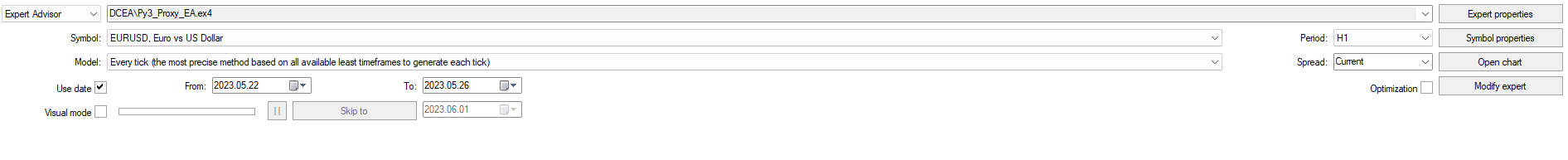
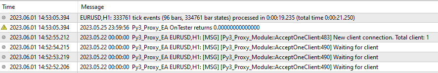
After you started the test, the EA on the MT4 side will be started and wait for the python client to connect. You can then start the python EA also.

If everything is alright, you will see the neural network is ready to use.
Conclusion
This is just the first try of the CNN approach, the model is not accurate enough to provide any good result. In this post, we have tried to link the python and MT4 together and leverage the CNN ability on live trading. Going forward, we will start to use different CNN model to see if you can achieve a better trading perform on both backtest and live trading.
Reference
Practical application of neural networks in trading


