Data Science and ML (Part 22): Leveraging Autoencoders Neural Networks for Smarter Trades by Moving from Noise to Signal

What are Autoencoders?

Autoencoders are unsupervised artificial neural networks. In its simplest form, An autoencoder is a neural network that tries two things. It compresses its input data into lower dimension then it tries to use this lower dimensional representation of the data to recreate the original input.

Suppose you have a blurred cat image passed to the autoencoder, this image will be compressed and decompressed back to its original state losing some of its noisy/blurred pixels along the process to end up with a clear image of a cat.

In this article, we will see how we can use an autoencoder neural network in the financial space to help us remove noise in the market so that we can discover trading opportunities.

This article is an easy read if you have a basic understanding of ONNX, PCA, and Neural Networks in general.

An Autoencoder consists of two parts:

1. An Encoder takes the input data and compresses it into lower-dimensional latent representation, capturing the essential features.
2. A Decoder receives the latent representation and attempts to reconstruct the original input data as accurately as possible.

Advantages of Autoencoders:

• They can be useful for dimensionality reduction tasks since they can learn a compressed representation of the forex trading data, which is useful for tasks like feature extraction, data compression, and visualization in high-dimensional datasets.
• By trying to reconstruct the input data, the autoencoder learns essential features and removes noise or irrelevant information. These learned features can be beneficial for other machine-learning tasks like classification or anomaly detection.
• Since they are unsupervised, they can discover hidden patterns in the trading data without human interaction.
• The learned latent representation from an autoencoder can be used as pre-trained features for other models, potentially improving their performance.

What are they Made up of?

Let us dissect autoencoders and observe what are they made up of and what makes them special.

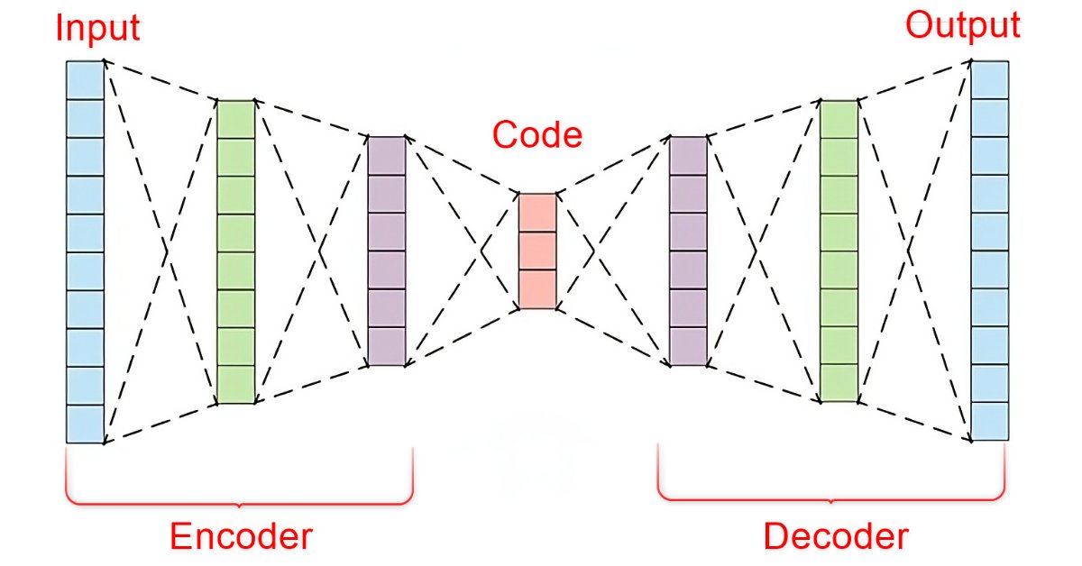
At the core of an autoencoder, there is an artificial neural network which consists of three parts.

1. The Encoder
2. The Embedding vector/latent layer
3. The Decoder

The left part of the neural network is called an encoder, Its job is to transform the original input data into lower dimensional representation.

The middle part of the neural network is called the latent layer or Embedding vector, its role is to compress the input data into lower dimensional data, This layer is expected to have fewer neurons than both the encoder and the decoder.

The right part of this neural network is called the decoder, Its job to to recreate the original input using the output of the encoder In other words, It tries to reverse the encoding process.

This is fascinating because the decoder tries to recreate a higher dimensional data from lower dimensional data returned by the encoder. Something like trying to build a house by looking at a picture of one.

This forces information loss which is key to this whole process working. By making it so that the decoder has imperfect information and training the whole network to minimize the construction error. During training the encoder and decoder are forced to work together to minimize the construction error.

Construction error is the difference between the attempted recreation and the original input data.

If we do not have an information loss between the encoder and the decoder then the network would simply learn to multiply the input by one and get a perfect reconstruction making the autoencoder useless. having an encoder with some degree of errors is crucial to this machine-learning technique, be sure not to overfit your model.

Both encoders and decoders are not limited to a single layer as can be seen in the Autoencoder architecture image shown above, It can contain multiple layers as seen in the below Python code where we have a list named hidden_dims for storing both encoder and decoder layers neurons.

Python:

class Autoencoder(Model):
  def __init__(self, input_dim, latent_dim, hidden_dims=[]):
    super(Autoencoder, self).__init__()

    self.encoder = tf.keras.Sequential()
    # Add hidden layers to the encoder (if any)
    for dim in hidden_dims:
      self.encoder.add(layers.Dense(dim, activation='relu'))
      self.encoder.add(layers.Dropout(0.5))

    # Define the latent layer
    self.encoder.add(layers.Dense(latent_dim, activation='relu'))

    # Decoder ( mirrored structure )
    self.decoder = tf.keras.Sequential()
    # Add hidden layers to the decoder (in reverse order)
    for dim in hidden_dims[::-1]:
      self.decoder.add(layers.Dense(dim, activation='relu'))
      self.decoder.add(layers.Dropout(0.5))

    # Define the output layer
    self.decoder.add(layers.Dense(input_dim, activation='sigmoid'))  #the output layer with dimensions matching the original input data

  def call(self, x):
    encoded = self.encoder(x)
    decoded = self.decoder(encoded)
    return decoded

Calling the class Autoencoder:

Python:

input_dim = dataset.shape[1]  # number of columns in the data
latent_dim = 5  # Dimension of latent layer
hidden_dims = [12, 10]

autoencoder = Autoencoder(input_dim, latent_dim, hidden_dims)

Below is how the architecture of the Autoencoder looks:

In the Autoencoder class, you have seen the use of RELU(Rectified Linear Unit) in both the encoder and the decoder. This activation function is widely used in most of the Autoencoders you will face there is an important reason for this.

RELU is computationally efficient, it avoids vanishing gradients and can learn sparse representations which are usually found in the trading data. Other variants of RELU such are GELU and Leaky RELU can be helpful when working with financial data.

Other popular activation functions such as Sigmoid and Hyperbolic Tangent(TANH) can be useful however one must understand their pros and cons before using them in trading data.

Sigmoid:

• Pros: Often used for image reconstruction where the output needs to be between 0 and 1 (representing pixel intensity).
• Cons: Might not be ideal for financial data as it can introduce vanishing gradients during backpropagation, especially in deep architectures.
  When sigmoid was applied to the Autoencoder the network failed to converge as it kept oscillating toward local the minima:
  

  Epoch 1/50
  110/110 ━━━━━━━━━━━━━━━━━━━━ 3s 5ms/step - loss: 0.4001 - val_loss: 0.3753
  Epoch 2/50
  110/110 ━━━━━━━━━━━━━━━━━━━━ 0s 4ms/step - loss: 0.3733 - val_loss: 0.3745
  Epoch 3/50
  110/110 ━━━━━━━━━━━━━━━━━━━━ 0s 4ms/step - loss: 0.3724 - val_loss: 0.3746
  Epoch 4/50
  110/110 ━━━━━━━━━━━━━━━━━━━━ 0s 4ms/step - loss: 0.3758 - val_loss: 0.3746
  Epoch 5/50
  110/110 ━━━━━━━━━━━━━━━━━━━━ 0s 4ms/step - loss: 0.3692 - val_loss: 0.3745
  Epoch 6/50
  110/110 ━━━━━━━━━━━━━━━━━━━━ 0s 4ms/step - loss: 0.3747 - val_loss: 0.3746
  Epoch 7/50
  110/110 ━━━━━━━━━━━━━━━━━━━━ 0s 4ms/step - loss: 0.3716 - val_loss: 0.3746
  Epoch 8/50
  110/110 ━━━━━━━━━━━━━━━━━━━━ 0s 4ms/step - loss: 0.3740 - val_loss: 0.3745
  Epoch 9/50
  110/110 ━━━━━━━━━━━━━━━━━━━━ 0s 4ms/step - loss: 0.3698 - val_loss: 0.3745
  Epoch 10/50
  110/110 ━━━━━━━━━━━━━━━━━━━━ 0s 4ms/step - loss: 0.3713 - val_loss: 0.3745
  Epoch 11/50
  110/110 ━━━━━━━━━━━━━━━━━━━━ 0s 4ms/step - loss: 0.3726 - val_loss: 0.3745
  Epoch 12/50
  110/110 ━━━━━━━━━━━━━━━━━━━━ 0s 4ms/step - loss: 0.3739 - val_loss: 0.3745
  Epoch 13/50
  110/110 ━━━━━━━━━━━━━━━━━━━━ 0s 4ms/step - loss: 0.3725 - val_loss: 0.3746
  Epoch 14/50
  110/110 ━━━━━━━━━━━━━━━━━━━━ 0s 4ms/step - loss: 0.3749 - val_loss: 0.3746

Tanh (Hyperbolic Tangent):

• Pros: Outputs range between -1 and 1, similar to sigmoid but with steeper gradients, potentially leading to faster convergence.
• Cons: Can still suffer from vanishing gradients in very deep networks.

These Sigmoid and TANH activation functions and others of their kind work best when used in the output layer of the decoder for the sake of reconstructing the input data as accurately as possible. In this context, the output of the autoencoder should resemble the original input. Since the input data is often normalized to the range [0, 1] or [-1, 1], depending on the preprocessing, the sigmoid activation function is commonly used to scale the output values to this range.

Python:

# Define the output layer
self.decoder.add(layers.Dense(input_dim, activation='sigmoid'))  #the output layer of the decoder with dimensions matching the original input data

Min-Max Scaler is your Friend

Autoencoders are simple to code and deploy however, they need to be given the right information and tools for them to work well. As we just seen why the choice of an activation function is crucial to this neural network type and so is the scaling technique.

Since we are using the RELU activation function which returns the value of zero when a value less than or equal to zero is given to it, otherwise it returns the given value ie. (x = 0 when x<=0 else x = x).

When you use Standard-Scaler, it centers the data by subtracting the mean and scales it to unit variance. This can push outliers with large positive values towards very negative values (potentially -1) during standardization. If a standardized value from an outlier becomes -1, when this negative value is passed the RELU activation in the encoder will always output 0 for that specific feature.

This can lead to a phenomenon called dying "RELU neurons" where some neurons in the encoder never get activated because of these negative input values. These dying RELU neurons can hinder learning in the encoder as they essentially become inactive and don't contribute to the encoding process most outliers or spikes in the trading data will be predicted flat mostly; see the below image where Standard-scaler was used.

 

To Address this Issue:

Try other normalization techniques such as the Min-Max scaler which scales data to a specific range between 0 and 1, potentially avoiding the creation of -1 values that causes RELU issues. However, considering the limitations of the Min-Max scaler, you can also explore the Robust scaler, which is less sensitive to outliers than the Standard scaler and might offer better scaling for RELU activations.

Also you might want to Consider using Leaky RELU (leaky_relu = 0.01x for x <= 0, relu = x for x > 0) instead of standard RELU. Leaky RELU allows a small non-zero gradient even for negative inputs, mitigating the dying RELU problem.

Training the Autoencoder

Now that we have discussed shortly the fundamentals of an Autoencoder let us train one and see how we can use it to help us for trading.

Python:

import sklearn
from sklearn.model_selection import train_test_split
from keras import optimizers
from keras.callbacks import EarlyStopping

x_train, x_test = train_test_split(dataset, test_size=0.3, random_state=42) #train test the data

# Normalizing the input data 

scaler = sklearn.preprocessing.MinMaxScaler()
x_train = scaler.fit_transform(x_train)
x_test = scaler.transform(x_test)

print(f"x_train {x_train.shape}.dtype({x_train.dtype}) x_test {x_test.shape}.dtype({x_test.dtype})")

# compile the autoencoder

input_dim = dataset.shape[1]
latent_dim = 32  # Dimension of latent space
hidden_dims = [256, 128, 64]

autoencoder = Autoencoder(input_dim, latent_dim, hidden_dims)

optimizer = optimizers.Adam(learning_rate=1e-5)
autoencoder.compile(optimizer=optimizer, loss=losses.MeanSquaredError())

early_stopping = EarlyStopping(monitor='val_loss', patience = 5, restore_best_weights=True) //stop the training process if 5 epochs have no change in loss
history = autoencoder.fit(x_train, x_train, epochs=50, shuffle=True, callbacks=[early_stopping], validation_data=(x_test, x_test), batch_size=64, verbose=1)

I chose to go with a complex neural network architecture [256, 128, 64] for the encoder a reverse arrangement of [64,128, 256] will be applied to the decoder, while having 32 neurons in the latent layer.

A neural network this complex has a higher chance of overfitting the training data, feel free to start with simpler architectures this is just an example. 

Outputs:

x_train (7000, 4).dtype(float64) x_test (3000, 4).dtype(float64)
Epoch 1/50
110/110 ━━━━━━━━━━━━━━━━━━━━ 3s 5ms/step - loss: 0.0669 - val_loss: 0.0636
Epoch 2/50
110/110 ━━━━━━━━━━━━━━━━━━━━ 0s 4ms/step - loss: 0.0648 - val_loss: 0.0608
Epoch 3/50
110/110 ━━━━━━━━━━━━━━━━━━━━ 0s 4ms/step - loss: 0.0624 - val_loss: 0.0550

....
....
....

Epoch 46/50
110/110 ━━━━━━━━━━━━━━━━━━━━ 0s 4ms/step - loss: 1.2096e-04 - val_loss: 1.0195e-04
Epoch 47/50
110/110 ━━━━━━━━━━━━━━━━━━━━ 0s 4ms/step - loss: 1.0758e-04 - val_loss: 9.7759e-05
Epoch 48/50
110/110 ━━━━━━━━━━━━━━━━━━━━ 0s 4ms/step - loss: 1.0923e-04 - val_loss: 9.4798e-05
Epoch 49/50
110/110 ━━━━━━━━━━━━━━━━━━━━ 1s 5ms/step - loss: 1.0243e-04 - val_loss: 9.0442e-05
Epoch 50/50
110/110 ━━━━━━━━━━━━━━━━━━━━ 1s 4ms/step - loss: 1.0222e-04 - val_loss: 8.7384e-05

Loss vs Iteration graph:

Let us pass the data to the Autoencoder and observe the outcome;

Python:

original_norm_data = scaler.transform(dataset)

new_data = autoencoder.call(original_norm_data)

new_data = scaler.inverse_transform(new_data) #return data to the original form 

print("original data\n",dataset,"\nnew data\n",new_data)

Outputs:

original data
 [[1.06507 1.06633 1.06497 1.06538]
 [1.06628 1.06685 1.06463 1.06508]
 [1.06771 1.06797 1.06599 1.06627]
 ...
 [0.99941 0.99996 0.9991  0.99916]
 [0.99687 0.99999 0.99646 0.99941]
 [0.99536 0.99724 0.99444 0.99687]] 
new data
 [[1.06612682 1.06676685 1.06537819 1.06605109]
 [1.06617137 1.06679912 1.06541834 1.06609218]
 [1.06742607 1.06804771 1.06668032 1.06736937]
 ...
 [0.99906356 1.00121275 0.9980908  0.99980352]
 [0.998204   1.00034005 0.9972261  0.99893805]
 [0.99581326 0.99789913 0.99494114 0.99651365]]

I decided to visualize the closing prices:

We can conclude that the new data passed through the autoencoder has some noise filtered and it is easy to detect the outliers just by looking at the chart. Now that we are sure it works let us discuss autoencoder applications and how we can finally use them in our MQL5-based programs.

Applications of Autoencoders

Autoencoders have been used in various fields and industries such as engineering, medicine field, entertainment, and much more for dimensionality reduction, feature learning, anomaly detection, in recommendation systems, and image denoising.

Dimensionality Reduction

Autoencoders excel at compressing high-dimensional data into lower-dimensional latent space. This is particularly valuable when dealing with datasets containing a large number of features, they capture the essential features in a more compact representation which can:

• Improve computational efficiency in subsequent machine-learning tasks by reducing the number of features to process. 
• Enhance visualization of high-dimensional data by allowing for dimensionality reduction techniques like Principal Component Analysis (PCA) to be applied to the learned latent space.

To achieve this task we need to use only the encoder part of our neural network. 

We need to modify the Autoencoder class by adding the build function which is supposed to be called shortly after the Autoencoder class is initiated. This method is useful for dynamically creating layers based on the shape of the input data, allowing you to delay the construction of layers until their shapes are known.

Python:

class Autoencoder(Model):
  def __init__(self, input_dim, latent_dim, hidden_dims=[]):
    super(Autoencoder, self).__init__()
    self.hidden_dims = hidden_dims
    self.input_dim = input_dim
    
    # Encoder
    self.encoder = tf.keras.Sequential(name='encoder') #give the encoder Sequential layer name=encoder
    # Decoder ( mirrored structure )
    self.decoder = tf.keras.Sequential(name='decoder') #give the decoder Sequential layer name=decoder
    
  def build(self):

    # Add hidden layers to the encoder (if any)
    for dim in hidden_dims:
      self.encoder.add(layers.Dense(dim, activation='relu'))
      self.encoder.add(layers.Dropout(0.5))

    # Define the latent layer
    self.encoder.add(layers.Dense(latent_dim, activation='relu'))
        
    # Add hidden layers to the decoder (in reverse order)
    for dim in hidden_dims[::-1]:
      self.decoder.add(layers.Dense(dim, activation='relu'))
      self.decoder.add(layers.Dropout(0.5))

    # Define the output layer
    self.decoder.add(layers.Dense(self.input_dim, activation='sigmoid'))  #the output layer with dimensions matching the original input data

  def call(self, x):
    encoded = self.encoder(x)
    decoded = self.decoder(encoded)
    return decoded

We also need to change a bit the way we call our class functions, as said earlier we are supposed to call the build function before compiling and training our neural network model. The order or calling the class methods is important!

Python:

# Instantiate the autoencoder and build the model
autoencoder = Autoencoder(input_dim, latent_dim, hidden_dims)
autoencoder.build()

optimizer = optimizers.Adam(learning_rate=1e-5)
autoencoder.compile(optimizer=optimizer, loss=losses.MeanSquaredError())

Now that we have the build function in place, we can finally extract both the encoder and the decoder neural networks separately soon after the Autoencoder has been trained successfully without errors.

Python:

# Extract Encoder
encoder_input = autoencoder.encoder.layers[0].input
encoder_output = autoencoder.encoder.get_layer(index=-1).output # the layer at index -1 is the last layer

# Define the encoder model
encoder_model = tf.keras.Model(inputs=encoder_input, outputs=encoder_output)

# Extract Decoder
decoder_input = autoencoder.decoder.layers[0].input
decoder_output = autoencoder.decoder.get_layer(index=-1).output # the layer at index -1 is the last layer

# Define the decoder model
decoder_model = tf.keras.Model(inputs=decoder_input, outputs=decoder_output)

Once we have the encoder we can pass the information and obtain the outcome matrix passed through the latent layer(space).

Python:

from sklearn.decomposition import PCA

# Fit & transform the encoded data 
encoded_data = encoder_model.predict(original_norm_data)
print("decoded data.shape: ",encoded_data.shape)

# Create PCA object
pca = PCA(n_components=encoded_data.shape[1])

reduced_data = pca.fit_transform(encoded_data)
print("pca reduced data.shape: ",reduced_data.shape)

print("explained var:\n",np.cumsum(pca.explained_variance_ratio_))

# Plotting the scree plot
plt.figure(figsize=(10, 6))
plt.plot(np.cumsum(pca.explained_variance_ratio_))
plt.xlabel('Number of Components')
plt.ylabel('Cumulative Explained Variance')
plt.title('Scree Plot')
plt.grid(True)
plt.show()

By assigning the number of columns encoded_data.shape[1] to the PCA components we can measure each feature explained variance and draw a scree plot which can help us understand the best number of components to apply to the PCA to shrink the data dimension.

313/313 ━━━━━━━━━━━━━━━━━━━━ 0s 1ms/step
decoded data.shape:  (10000, 32)
pca reduced data.shape:  (10000, 32)
explained var:
 [0.99623495 0.9989214  0.99982804 0.9999363  0.99996614 0.9999872
 0.99999297 0.9999953  0.9999972  0.9999982  0.9999987  0.9999991
 0.9999994  0.9999996  0.9999997  0.9999998  0.99999994 1.
 1.         1.         1.         1.         1.         1.
 1.         1.         1.         1.         1.         1.
 1.         1.        ]

By looking at the Cumulative Explained Variance we can observe explained variance ratios close to 1 mostly and 1 for some components. This implies that you might be able to achieve significant dimensionality reduction without losing much information.
The scree plot shows the elbow point at almost 2 components, which explains about 0.9989 total variance, this is the best number of components to reduce our data. Even 1 component should work fine as I couldn't see a major distinction between the components when I plotted them on one axis.

Next time the PCA class is called, it should be called with the value of 2 applied to it to get 2 components out of it.

# Create PCA object
pca = PCA(n_components=2)

reduced_data = pca.fit_transform(encoded_data)
print("pca reduced data.shape: ",reduced_data.shape)

Outcome:

pca reduced data.shape:  (10000, 2)

I decided to plot all 32 components from the latent layer in one axis. Only one feature was very much distinct from the others which looked almost the same on the chart this goes on to clarify a few components in this reduced data makes sense.

bar = [count+1 for count in range(reduced_data.shape[0])]

plt.figure(figsize = (7,10))
for col in range(reduced_data.shape[1]):
    plt.plot(bar,  reduced_data[:, col],label=f'feature {col}')
    
plt.xlabel("index")
plt.ylabel("feature")
plt.title("PCA encoded features")
plt.legend()
plt.savefig("pca-encoded features")

Components vs Index plot:

Applying PCA to the autoencoder's latent space offers more control over the reduction process compared to directly applying PCA to the original high-dimensional data not to mention it helps reduce unnecessary noise in the data along the process.

An elephant in the room:

In the example discussed we reduced the dimension of all the input data this may not be ideal when you want to apply the data reduced after PCA in predictive models, in that case, you might need to apply PCA to independent variables only.

But before we can use this autoencoder we created to reduce noise from the trading data in MetaTrader 5 as another Autoencoder application, we need to save it to ONNX format.

Saving the Autoencoder Model to ONNX format

We already extracted both the encoder and the decoder before applying them for dimension reduction converting and saving them in ONNX format should be easy. Let us start with the encoder model as we will save both of them separately.

Python:

import tf2onnx
import onnx
import os

output_path = os.path.join('/kaggle/working/',"encoder.eurusd.h1.onnx")

# saving the encoder for MetaTrader 5

input_signature = [tf.TensorSpec(encoder_input.shape, tf.float16, name='x_inputs')] #onnx input signature
# Use from_function for tf functions
onnx_model, _ = tf2onnx.convert.from_keras(encoder_model, input_signature, opset=13)
onnx.save(onnx_model, output_path)

The input_signature for ONNX helps to avoid errors with the latest versions of TensorFlow and ONNX as it helps clarify the input names for our .onnx file when loading a model of this format in MetaTrader 5.

Saving the decoder model:

Python:

# saving the decoder

output_path = os.path.join('/kaggle/working/',"decoder.eurusd.h1.onnx")

input_signature = [tf.TensorSpec(decoder_input.shape, tf.float16, name='decoder_inputs')] #onnx input signature

onnx_model, _ = tf2onnx.convert.from_keras(decoder_model, input_signature, opset=13) #conver keras model to onnx
onnx.save(onnx_model, output_path)

In the article Overcoming ONNX Integration Challenges, I tackled the problem of integrating the same dimension reduction and scaling techniques available for both Python and mql5 programming language for precision, but I found an easy solution for mitigating the scaling problem.

Saving the Scaler:

Using the same scaler in Python and mql5 is crucial. I can't stress enough how important this is.

Python:

scaler.data_min_.tofile("minmax_min.bin")
scaler.data_max_.tofile("minmax_max.bin")

We save the Min-Max scaler information arrays to simple binary files that we can include in our MetaTrader 5 indicator. After saving them under the MQL5\Files folder.

MQL5 (AutoEncoder Indicator.mq5):

//Load both the encoder_model and the decoder_model
#resource "\\Files\\encoder.eurusd.h1.onnx" as uchar encoder_onnx[];
#resource "\\Files\\decoder.eurusd.h1.onnx" as uchar decoder_onnx[];

// Load the MinMax scaler also
#resource "\\Files\\minmax_min.bin" as double min_values[];
#resource "\\Files\\minmax_max.bin" as double max_values[];

Reducing Noise from the Trading Data

The Autoencoder can remove noise from the data as seen in various different aspects such as removing noise from images, we are yet to prove this in the financial data. Looking at the image for the close prices and the new close prices it is clear that the Auto-encoded close price values are less noisy, Lets make an indicator to help us draw the candles for the new OHLC provided by the Autoencoder.

MQL5 (AutoEncoder Indicator.mq5):

#property indicator_chart_window
#property indicator_plots 1
#property indicator_buffers 5

input bool show_bars = true;
input bool show_bullish_bearish = false;

//--- plot Candle
#property indicator_label1  "autoencoded open; high; low; close"
#property indicator_type1   DRAW_COLOR_CANDLES
#property indicator_color1  clrRed, clrGray
#property indicator_style1  STYLE_SOLID
#property indicator_width1  1

We need to make an Autoencoder class to make it easier to use the loaded ONNX models in MQL5 as if we are using them in Python.

MQL5(Autoencoder-onnx.mqh):

class CAutoEncoderONNX
  {
protected:

   bool initialized;
   long onnx_handle;
   void PrintTypeInfo(const long num,const string layer,const OnnxTypeInfo& type_info);
   long inputs[], outputs[];
   
   void replace(long &arr[]) { for (uint i=0; i<arr.Size(); i++) if (arr[i] <= -1) arr[i] = UNDEFINED_REPLACE; }
   
public:
                     CAutoEncoderONNX(void);
                    ~CAutoEncoderONNX(void);
                     
                     bool Init(const uchar &onnx_buff[], ulong flags=ONNX_DEFAULT); //load the onnx model from a resource uchar array
                     bool Init(string onnx_filename, uint flags=ONNX_DEFAULT); //load the onnx model from a .onnx file 
                     
                     matrix predict(const matrix &x); //passing inputs for either the encoder or the decoder to the outputs in matrix form
                     vector predict(const vector &x); //passing inputs for either the encoder or the decoder to the outputs in matrix form
  };

Instantiating the class CAutoEncoderONNX for each model separately as they are:

MQL5 (AutoEncoder Indicator.mq5):

#include <Autoencoder-onnx.mqh>
#include <MALE5\preprocessing.mqh>

CAutoEncoderONNX encoder_model; //for the encoder model
CAutoEncoderONNX decoder_model; //for the decoder model
MinMaxScaler *scaler; //Python-like MinMax scaler

Initializing the models:

MQL5 (AutoEncoder Indicator.mq5):

//+------------------------------------------------------------------+
//| Custom indicator initialization function                         |
//+------------------------------------------------------------------+
int OnInit()
  {
   if (!encoder_model.Init(encoder_onnx)) //initializing the encoder
     return INIT_FAILED;
   
   if (!decoder_model.Init(decoder_onnx)) //initializing the decoder
     return INIT_FAILED;
   
   scaler = new MinMaxScaler(min_values, max_values); //Load the Minmax scaler saved in python
     
//---
   return(INIT_SUCCEEDED);
  }

To obtain the predictions out of the model we are going to pass raw data to the encoder and then pass the outcome to the decoder for final output. Remember! in Python, we had two separate models passed one after the other in the call function.

Python:

class Autoencoder(Model):
...
...

  def call(self, x):
    encoded = self.encoder(x)
    decoded = self.decoder(encoded)
    return decoded

Let us see this in action in mql5:

MQL5 (AutoEncoder Indicator.mq5):

//+------------------------------------------------------------------+
//| Custom indicator iteration function                              |
//+------------------------------------------------------------------+
int OnCalculate(const int rates_total,
                const int prev_calculated,
                const datetime& time[],
                const double& open[],
                const double& high[],
                const double& low[],
                const double& close[],
                const long& tick_volume[],
                const long& volume[],
                const int& spread[])
  {
//---
   
   int start = prev_calculated;
   if(start>=rates_total)
      start = rates_total-1;
   
   
   vector encoded_data = {}, decoded_data = {};
   for(int i = start; i<rates_total; i++)
     {
        vector x_inputs = {open[i], high[i], low[i], close[i]};
        
        x_inputs = scaler.transform(x_inputs); //Normalize the input data, important!
        encoded_data = encoder_model.predict(x_inputs); //encode the data
        decoded_data = decoder_model.predict(encoded_data); //decode the data
        
        decoded_data = scaler.inverse_transform(decoded_data); //return data to its original state  
          
        open_candle[i]= decoded_data[0];
        high_candle[i]= decoded_data[1];
        low_candle[i]=  decoded_data[2];
        close_candle[i]=decoded_data[3];
        
        // Set upper and lower body colors based on the gradient
        
        if (close_candle[i]>open_candle[i])
         {
           color_buffer[i] = 1.0; //Draw gray for bullish candle
         }
        else
         {
          color_buffer[i] = 0.0; //draw red when there was a bearish candle
         }
                         
        if (MQLInfoInteger(MQL_DEBUG))
         Comment(StringFormat("plotting [%d/%d] OPEN[%.5f] HIGH[%.5f] LOW[%.5f] CLOSE[%.5f]",i,rates_total,open_candle[i],high_candle[i],low_candle[i],close_candle[i]));
     }
     
//--- return value of prev_calculated for next call
   return(rates_total);
  }

Indicator plot:

From my observation, the candlesticks made by the Autoencoder have almost the same body size and the difference between the lower price and higher prices is high and almost the same for all the candles.

Most candles are bearish market in red, and very few candles are bullish ones in gray color.

To make this indicator appear well on the chart we can fill the space between the lower and the higher price of the candle. For both bullish and bearish candles.

MQL5 (AutoEncoder Indicator.mq5):

  if (close_candle[i]>open_candle[i])
   {
     color_buffer[i] = 1.0; //Draw gray for bullish candle

     close_candle[i] = high_candle[i];
     open_candle[i] = low_candle[i];
   }
  else
   {
     color_buffer[i] = 0.0; //draw red when there was a bearish candle
    
     close_candle[i] = low_candle[i];
     open_candle[i] = high_candle[i];
   }

Indicator plot:

We can give our indicator an option to distinguish between bullish and bearish candles based on the actual open and close prices from the market.

MQL5 (AutoEncoder Indicator.mq5):

if (show_bullish_bearish)
 {
  if (close[i]>open[i])
   color_buffer[i] = 1.0;
  else
    color_buffer[i] = 0.0;
 }

Indicator plot:

We also have the option to hide the original candles and go with only the new candles made with the autoencoder.

Disadvantages of Autoencoders

Autoencoders, like all machine-learning models, come with their own set of challenges:

1. Imperfect Data Reconstruction
   Autoencoders try to recreate data after compressing it. Sometimes, they don't do a great job, leading to errors in reconstructing the original data. This is a problem if you need a very accurate recreation of the original data.

2. Hard to Understand
   The compressed data formats autoencoders produce can be tricky to interpret. It's often not clear what features of the data the autoencoder has managed to capture, which makes it hard to explain how the model works.

3. Sensitive to Noise
   Autoencoders aim to highlight main patterns in data but may struggle with noise and outliers. This can result in poor reconstruction and biased features, which isn't ideal.

4. Dimensionality Bottleneck
   The middle layer of an autoencoder, where data gets compressed, can sometimes be too small. If it doesn't have enough dimensions, it might not capture all the important information for what you need to do. Choosing the right size for this layer is key and depends on what you're trying to achieve.

5. Expensive to Train
   Training deep autoencoders, especially on large datasets, can use a lot of computing power. This is important to keep in mind if you have limited resources or time.

6. Not Great for All Tasks
   Autoencoders might not be the best choice for tasks like classification or regression, where working directly with the input data could be more effective.

7. Risk of Overfitting
   Using complex models for simple problems can lead to overfitting, where the model learns the training data too well but performs poorly on new, unseen data.

Final Thoughts

Autoencoders can be a great tool for reducing the noise in the forex market as seen in the indicator we ended up with less noisy candlesticks that still reflect the market, They could either be better or worse than the original candlesticks, These new candlesticks give us a different perspective of the market.

Feel free to explore the new candlesticks by extracting signals from patterns and building trading strategies on them.

Peace out.

Attachments Table: 

File	Description & Usage
Include\MatrixExtend.mqh	Has additional functions for matrix manipulations.
Include\ preprocessing.mqh	The library for pre-processing raw input data to make it suitable for machine-learning model usage.
Indicators\ AutoEncoder Indicator.mq5	The main indicator file. It deploys the discussed autoencoder and draws candles on the outcome predictions.
Include\ Autoencoder-onnx.mqh	A library for loading a machine-learning model in ONNX format and interpreting the outcomes.
Files\...	Save these files under the MQL5\Files folder
autoencoders.ipynb	Python Jupyter notebook for running all the Python code discussed