Alternative risk return metrics in MQL5

Introduction

All traders hope to maximize the percentage return on their investment by as much as possible, however higher returns usually come at a higher risk. This is the reason why risk adjusted returns are the main measure of performance in the investment industry. There are many different measures of risk adjusted return, each one with its own set of advantages and disadvantages. The Sharpe ratio is a popular risk return measure famous for imposing unrealistic preconditions on the distribution of returns being analyzed. This has inevitably lead to the development of alternative performance metrics that seek to provide the same ubiquity of the Sharpe ratio without its shortcommings. In this article we provide the implementation of alternative risk return metrics and generate hypothetical equity curves to analyze their characteristics.

Simulated equity curves

In order to ensure  interpretability we will use SP 500 data as the basis for a simulated trading strategy. We will not use any specific trading rules, instead we employ random numbers to generate equity curves and corresponding  returns series. The initial capital will be standardized to a configurable amount. Random numbers will be defined by a  seed so that anyone who wants to reproduce the experiments can do so.

Visualizing equity curves

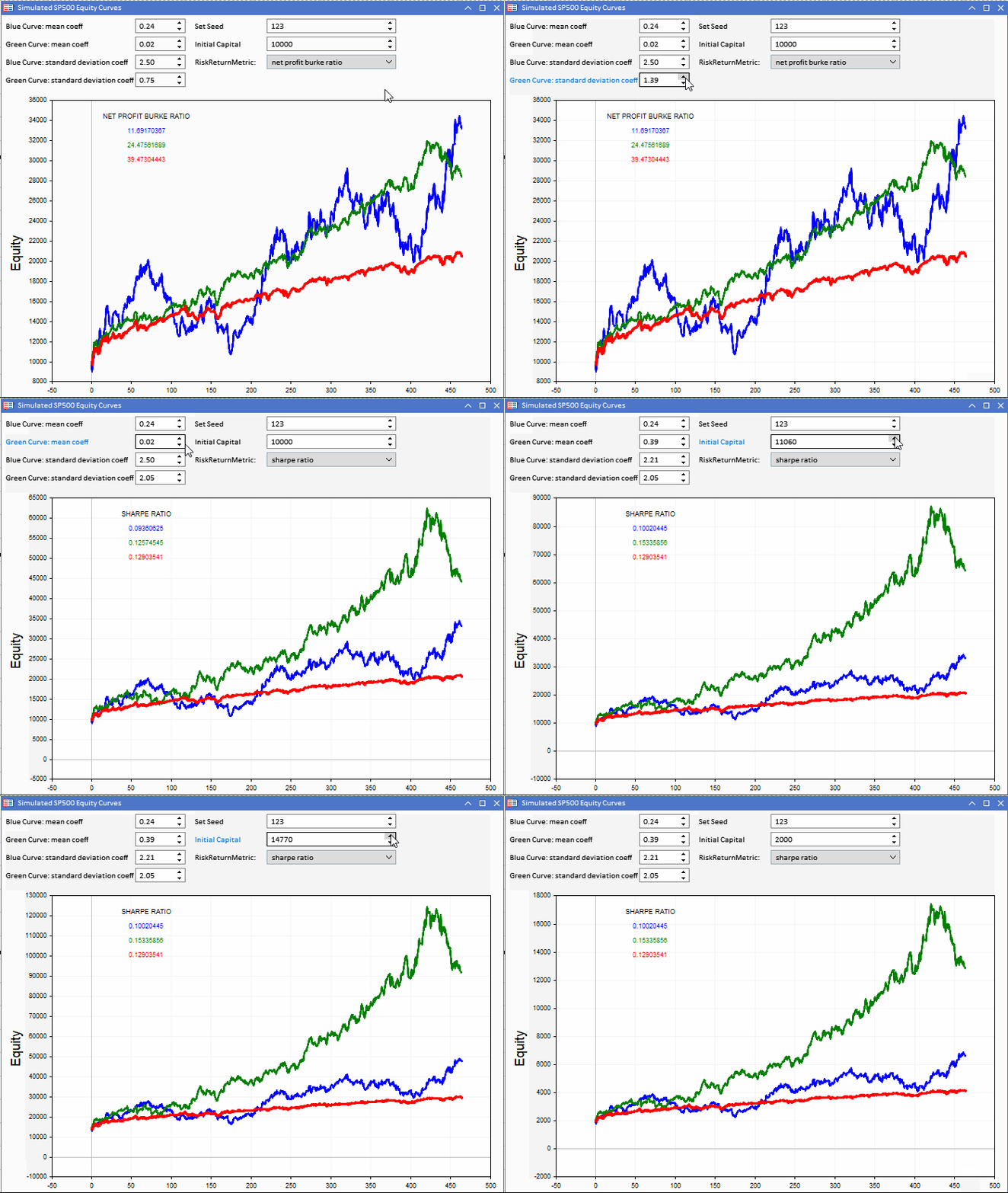
The graphic below represents a Metatrader 5 (MT5) application implemented as an Expert Advisor (EA), that displays three equity curves. The red equity curve is the benchmark from which the blue and green equity curves are derived. The benchmark can be altered by configuring the initial capital. Adjustable from the application.  

Equity curves will be created based on the benchmark series. Each one is defined by a random componet that can be controlled through two adjustable constants. The mean coefficient and a standard deviation coeffecient. These in combination with the standard deviation of benchmark returns, determine the parameters for the normaly distributed random numbers used to generate two hypothetical equity curves.   

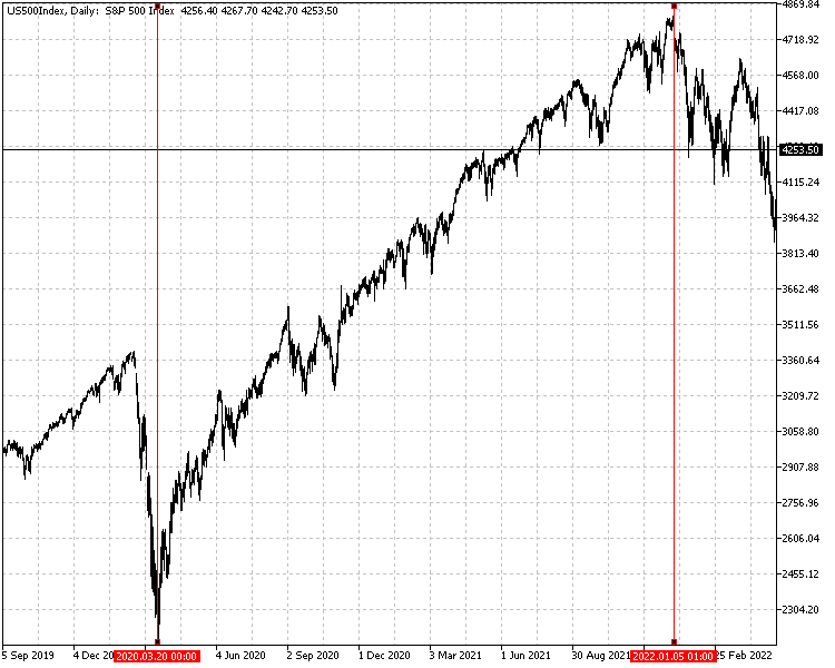
We first calculate the returns using SP 500 daily close prices from the period between 20 March 2020 and 5 January 2022, inclusive. The equity curve is built from the series of returns. With the series that define the equity and returns we will compare the performance results calculated along with the appearance of a given equity curve.

The code for the application is attached to the article.

Drawdown ratios

Drawdown represents the largest amount of equity that a strategy lost between any two points in time. This value gives an indication of the risk that a strategy took on to accomplish its gains, if any were attained. When  a series made up of an arbitrary number of the highest drawdowns is tallied and aggregated, the result can be used as a measure of variability.

Burke Ratio

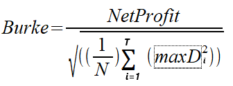
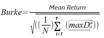
In 1994 Burke wrote a paper titled "A sharper sharpe ratio" , which introduced the Burke ratio as an alternative to the familiar Sharpe ratio. The Burke ratio substitutes the denominator in the Sharpe ratio formula for the squared sum of a specified number of the highest absolute drawdowns. The numerator can either be the mean return or the absolute monetary return of the strategy/portfolio, ie ,net profit. We will have a look at the two versions of the calculation. We distinguish the two versions as the net profit based Burke Ratio and the mean returns Burke Ratio. The formulae are given below.

MaxD is the series of the largest T absolute drawdowns calculated from the equity values. N represents the number of equity values used in the calculation.

The net profit Burke Ratio is implemented as the netprofit_burke() function. The function requires an array of equity values describing the equity curve as well as an integer value denoting the number of the highest drawdowns to consider in the computation.

//+------------------------------------------------------------------+
//|Net profit based Burke ratio                                      |
//+------------------------------------------------------------------+
double netprofit_burke(double &in_ec[],int n_highestdrawdowns=0)
  {
   double outdd[];
   double sumdd=0;
   int insize=ArraySize(in_ec);

   if(n_highestdrawdowns<=0)
      n_highestdrawdowns=int(insize/20);

   if(MaxNDrawdowns(n_highestdrawdowns,in_ec,outdd))
     {
      for(int i=0; i<ArraySize(outdd); i++)
        {
         sumdd+=(outdd[i]*outdd[i]);
        }
      return (in_ec[insize-1]-in_ec[0])/(MathSqrt((1.0/double(insize)) * sumdd));
     }
   else
      return 0;
  }

When the default value of zero is specified, the function uses the formula N/20 to set the number of drawdowns to consider, where N is the size of the equity array.

To collect the specified number of drawdowns, MaxNDradowns() function is enlisted. It outputs a series of the highest absolute drawdowns arranged in ascending order.

//+------------------------------------------------------------------+
//|Maximum drawdowns function given equity curve                     |
//+------------------------------------------------------------------+
bool MaxNDrawdowns(const int num_drawdowns,double &in_ec[],double &out_dd[])
  {
   ZeroMemory(out_dd);

   ResetLastError();

   if(num_drawdowns<=0)
     {
      Print("Invalid function parameter for num_drawdowns ");
      return false;
     }
   double u[],v[];

   int size = ArraySize(in_ec);

   if((ArrayResize(v,(size*(size-1))/2)< int((size*(size-1))/2))||
      (ArraySize(out_dd)!=num_drawdowns && ArrayResize(out_dd,num_drawdowns)<num_drawdowns))
     {
      Print(__FUNCTION__, " resize error ", GetLastError());
      return false;
     }

   int k=0;
   for(int i=0; i<size-1; i++)
     {
      for(int j=i+1; j<size; j++)
        {
         v[k]=in_ec[i]-in_ec[j];
         k++;
        }
     }

   ArraySort(v);

   for(int i=0; i<k; i++)
     {
      if(v[i]>0)
        {
         if(i)
           {
            if(!ArrayRemove(v,0,i))
              {
               Print(__FUNCTION__, " error , ArrayRemove: ",GetLastError());
               return false;
              }
            else
               break;
           }
         else
            break;
        }
     }

   size=ArraySize(v);

   if(size && size<=num_drawdowns)
     {
      if(ArrayCopy(out_dd,v)<size)
        {
         Print(__FUNCTION__, " error ", GetLastError());
         return false;
        }
      else
         return (true);
     }


   if(ArrayCopy(out_dd,v,0,size-num_drawdowns,num_drawdowns)<num_drawdowns)
     {
      Print(__FUNCTION__, " error ", GetLastError());
      return false;
     }


   return(true);

  }

The Burke ratio computation that uses mean returns as the numerator is implemented as the meanreturns_burke function and has similar input parameters.

//+------------------------------------------------------------------+
//|Mean return based Burke ratio                                     |
//+------------------------------------------------------------------+
double meanreturns_burke(double &in_ec[],int n_highestdrawdowns=0)
  {
   double outdd[];
   double rets[];

   double sumdd=0;
   int insize=ArraySize(in_ec);

   if(ArrayResize(rets,insize-1)<insize-1)
     {
      Print(__FUNCTION__," Memory allocation error ",GetLastError());
      return 0;
     }

   for(int i=1; i<insize; i++)
      rets[i-1] = (in_ec[i]/in_ec[i-1]) - 1.0;

   if(n_highestdrawdowns<=0)
      n_highestdrawdowns=int(insize/20);

   if(MaxNDrawdowns(n_highestdrawdowns,in_ec,outdd))
     {
      for(int i=0; i<ArraySize(outdd); i++)
         sumdd+=(outdd[i]*outdd[i]);
      return MathMean(rets)/(MathSqrt((1.0/double(insize)) * sumdd));
     }
   else
      return 0;
  }

Net profit to maximum drawdown ratio

The Burke ratio formula that uses net profit as the numerator is similar to the Netprofit to Maximum Drawdown ratio (NPMD). The difference is in the use of the single highest drawdown in the calculation of the NPMD ratio.

NPMD calculation is implemented as the netProfiMaxDD() function, requiring the array of equity values as input.

//+------------------------------------------------------------------+
//|Net profit to maximum drawdown ratio                              |
//+------------------------------------------------------------------+
double netProfiMaxDD(double &in_ec[])
  {
   double outdd[];
   int insize=ArraySize(in_ec);

   if(MaxNDrawdowns(1,in_ec,outdd))
      return ((in_ec[insize-1]-in_ec[0])/outdd[0]);
   else
      return 0;
  }

Drawdown based ratios were introduced to address some of the criticisms levied against the Sharpe ratio. The calculations do not penalize abnormal or large gains and most importantly are non-parametric. Although advantageous, the use of absolute drawdowns in the denominator makes both the Burke and NPMD ratios favour strategies with relatively mild downward spikes.

Refering to the equity curve visualization tool. The blue curve has the highest returns but it scores lower than the rest.

The benchmark values for both ratios emphasize just how misleading the metrics can be when used to compare the performance of strategies. The benchmark ratios are significantly higher despite the other curves delivering more in real returns.

Using absolute drawdowns can over emphasize risk, relative to using the distribution of negative returns as is the case with the Sharpe ratio.

Comparing the Sharpe scores, we see that the green curve has the highest, with much less of a difference between the simulated strategy results.

Drawdown ratios interpretation

The higher the Burke or NPMD ratio, the better the risk-adjusted performance of the investment strategy. It means the strategy is generating higher returns compared to the risk taken.

- If the Burke or NPMD ratio is greater than 0, it suggests that the investment strategy is providing excess return compared to the calculated risk.

- If the Burke or NPMD ratio is less than 0, it indicates that the investment strategy is not generating sufficient excess return compared to the risk taken.

Partial moment ratios

Partial moment based ratios are another attempt at an alternative to Sharpe Ratio. They are based on the statistical concept of semi variance and provide insights into how well a strategy is performing in terms of downside risk (negative returns) compared to upside potential (positive returns).To calculate partial moment ratios, we first need to determine the partial gain and partial loss. These values are derived by identifying a threshold return level, usually the minimum acceptable return or the risk-free rate, and calculating the difference between the actual return and the threshold return for each observation.

The calculation can ignore differences that are either above the threshold for the lower partial moment or below threshold for the higher partial moment (HPM). The lower partial moment (LPM) measures the squared deviations of returns that fall below the threshold, while the higher partial moment (HPM) measures the squared deviations of returns that exceed the threshold. Partial moments present an alternative perspective on risk compared to drawdown ratios, by focusing on the risk associated with returns that are either below or above a specific threshold.

Below are formulae for the LPM and HPM respectively:

Where thresh is the threshold , x is an observed return and max determines the maximum value between the resulting difference and zero before being raised to the power of n. n defines the degree of a partial moment. When n=0 , the LPM becomes the probability that an observation  is less than the threshold and HPM gives the probability it is above. N is the number of observed returns. Two partial moment ratios we will look at are the generalized Omega and the Upside Potential Ratio (UPR).

Omega

The generalized Omega is defined by an single n degree term and a threshold value which defines the LPM used in the calculation.

The omega() function implements the computation of the Omega ratio by taking as input an array of returns. The function uses a degree 2 lower partial moment, with the threshold returns taken as zero.

//+------------------------------------------------------------------+
//|omega ratio                                                       |
//+------------------------------------------------------------------+
double omega(double &rt[])
  {
   double rb[];

   if(ArrayResize(rb,ArraySize(rt))<0)
     {
      Print(__FUNCTION__, " Resize error ",GetLastError());
      return 0;
     }

   ArrayInitialize(rb,0.0);

   double pmomentl=MathPow(partialmoment(2,rt,rb),0.5);

   if(pmomentl)
      return MathMean(rt)/pmomentl;
   else
      return 0;
  }

Upside potential ratio

The UPR uses two n degree terms (n1 and n2 in the formula) and a threshold. n1 determines the HPM degree in the numerator and n2 specifies the LPM degree of the denominator.

Similar to the implementation of the Omega performance metric,  the upsidePotentialRatio() function computes the UPR ratio. The computation also uses degree 2 partial moments, and threshold returns defined as zero.

//+------------------------------------------------------------------+
//|Upside potential ratio                                            |
//+------------------------------------------------------------------+
double upsidePotentialRatio(double &rt[])
  {
   double rb[];

   if(ArrayResize(rb,ArraySize(rt))<0)
     {
      Print(__FUNCTION__, " Resize error ",GetLastError());
      return 0;
     }

   ArrayInitialize(rb,0.0);

   double pmomentu=MathPow(partialmoment(2,rt,rb,true),0.5);
   double pmomentl=MathPow(partialmoment(2,rt,rb),0.5);
   if(pmomentl)
      return pmomentu/pmomentl;
   else
      return 0;
  }

Partial moment calculations are implemented in the partialmoment() function. It requires as input the degree of the moment as an unsigned integer,  two arrays of double type and boolean value. The first array should contain the observed returns and the second the threshold or benchmark returns used in the calculation. The boolean value determines the type of partial moment to be calculated, either true for the  higher partial moment and false for the lower partial moment.

//+------------------------------------------------------------------+
//|Partial Moments                                                   |
//+------------------------------------------------------------------+
double partialmoment(const uint n,double &rt[],double &rtb[],bool upper=false)
  {
   double pm[];
   int insize=ArraySize(rt);

   if(n)
     {
      if(ArrayResize(pm,insize)<insize)
        {
         Print(__FUNCTION__," resize error ", GetLastError());
         return 0;
        }

      for(int i=0; i<insize; i++)
         pm[i] = (!upper)?MathPow(MathMax(rtb[i]-rt[i],0),n):MathPow(MathMax(rt[i]-rtb[i],0),n);
      return MathMean(pm);
     }
   else
     {
      int k=0;
      for(int i=0; i<insize; i++)
        {
         if((!upper && rtb[i]>=rt[i]) || (upper && rt[i]>rtb[i]))
           {
            ArrayResize(pm,k+1,1);
            pm[k]=rt[i];
            ++k;
           }
         else
            continue;
        }

      return MathMean(pm);

     }

  }

Looking at the Omega and UPR ratios of our equity curves we notice the similarity in rating with that of the Sharpe ratio.

Again consistency is favoured over the more volatile equity curves. Omega specifically looks like a viable alternative to the Sharpe ratio.

Partial moment ratio interpretation

Omega is much more straight forward when it comes to its interpretation relative to the UPR. The higher omega is the better. Negative values indicate money losing strategies with positive values suggesting performance that delivers excess returns relative to the risk take.

The UPR on the other hand can be a bit of an oddball when it comes to interpretation , have a look at some simulated equity curves with diverging performance profiles.

The blue equity cure shows negative returns yet the UPR result is positive. Even more odd are the results from the green and red equity curves. The curves themselves are almost similar with the green equity curve producing the better returns yet the UPR value is less than that of the red curve.

Regression analysis of returns - Jensen's Alpha

Linear regression enables construction of a line that best fits a data set. Regression based metrics therefore measure the linearity of equity curves. Jensen's Alpha computes the value of alpha in the standard regression equation. It quantifies the relationship between benchmark returns and the observed returns.

To calculate the value of alpha we can use the least squares fit method. The function leastsquarefit() function takes as input two arrays that define the response and the predictor. In this context the response would be the an array of observed returns and the predictor is the array of benchmark returns. The function outputs the alpha and beta values whose references should be supplied when calling the function.

//+------------------------------------------------------------------+
//|linear model using least squares fit y=a+bx                       |
//+------------------------------------------------------------------+
double leastsquaresfit(double &y[],double &x[], double &alpha,double &beta)
  {
   double esquared=0;

   int ysize=ArraySize(y);
   int xsize=ArraySize(x);

   double sumx=0,sumy=0,sumx2=0,sumxy=0;

   int insize=MathMin(ysize,xsize);

   for(int i=0; i<insize; i++)
     {
      sumx+=x[i];
      sumx2+=x[i]*x[i];
      sumy+=y[i];
      sumxy+=x[i]*y[i];
     }

   beta=((insize*sumxy)-(sumx*sumy))/((insize*sumx2)-(sumx*sumx));
   alpha=(sumy-(beta*sumx))/insize;

   double pred,error;

   for(int i=0; i<insize; i++)
     {
      pred=alpha+(beta*x[i]);
      error=pred-y[i];
      esquared+=(error*error);
     }

   return esquared;

  }

Applying Jensen's Alpha to our simulated equity curves, we get a measure of the linearity of the green and blue equity curves relative to the benchmark (red equity curve).

This is the first metric that rates the blue equity curve as the best performing strategy. This metric usually rewards good performance when the bechmark returns are bad. It is possible for Jensen's alpha to indicate positive returns even if absolute returns are negative. This can happen when the absolute benchmark returns are simply worse than the returns being studied. So be careful when using this metric.

Jensen's Alpha interpretation

If Jensen's Alpha is positive, it suggests that the portfolio/strategy has generated excess returns compared to a benchmark, indicating outperformance after considering its risk level. Otherwise, if Jensen's Alpha is negative, it implies that the strategy has underperformed relative to the benchmark returns.

Besides the alpha value, the beta value from the least squares computation provides a measure of the sensitivity of returns relative to the benchmark. A beta of 1 indicates that the strategy's returns move in sync with the benchmark. A beta less than 1 suggests the equity curve is less volatile than that of the  benchmark, while a beta greater than 1 indicates higher volatility.

Conclusion

We have described the implementation of a few risk adjusted return metrics that could be used to as alternatives to the Sharpe Ratio. In my opinion, the best candidate is the omega metric. It provides the same advantages of the Sharpe ratio without any expectation of normality in the distribution of returns. Though, it should also be noted that its better to consider multiple strategy performance metrics when making investment decisions. One will never be able to provide a complete picture of expected risk or returns. AlsoRemember, most risk return metrics provide retrospective measures, and historical performance does not guarantee future results. Therefore, it's important to consider other factors like investment objectives, time horizon, and risk tolerance when assessing investment options.

The source code for all metrics are contained in PerformanceRatios.mqh. It should be noted that none of the implementations produce annualized figures. The attached zip file also contains the code for the application used to visualize our simulated equity curves. It was implemented using the EasyAndFastGUI library which is available at the  mql5.com codebase. The library is not attached, with the article. What is attached is source code of the EA and a working compiled version.

FileName	Description
Mql5\Files\sp500close.csv	an attached csv file of SP500 close prices used in the calculation of the equity curves
Mql5\Include\PerformanceRatios.mqh	include file that contains the definition of all the performance metrics described in the article
Mql5\Experts\EquityCurves.mq5	Expert advisor source code for the visualization tool, for it to compile it requires the easy and fast gui available in the codebase
Mql5\Experts\EquityCurves.ext	This is the compiled version of the EA