Filtering and feature extraction in the frequency domain

Introduction

In the realm of financial markets, accurate prediction models are highly sought after. Reliable predictive models require meaningful and relevant information. In this article, we will explore the use of various digital filters applied in the frequency domain, as tools for feature extraction. We will go over some of the advantages and disadvantages of  analyzing time series converted to the frequency domain using the Discrete Fourier Transform (DFT). Three types of digital filters will be discussed: In-phase, in-quadrature and quadrature mirror filters. Emphasizing each type's utility in time series analysis. Finally, code will be presented that implements examples of each type.

Filtering in the frequency domain

In the article "Practical Implementation of Digital Filters in MQL5 for Beginners" the author, presented  digital filters applied in the time domain, through convolution. The series is multiplied with a unique set of weights of varying length, depending on the filter type and its parameters. The number of weights define a moving window that is convolved with corresponding series values as the filter is applied over the extent of the data. Moving averages also work in the same manner.

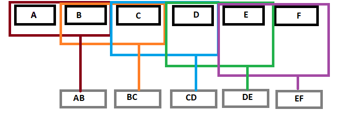
In this article, we will apply filters in the frequency domain. The basic steps involved are as follows:

1.  First the series is preprocessed in preparation of a DFT operation.
2.  The DFT is applied to the series using the Fast Fourier Transfrom algorithm (FFT).
3.  Next we manipulate the waveform of the series in whatever way we deem necessary. That is to say, a filter is applied, thereby modifying the original waveform of the series.
4.  An inverse DFT operation is done on the modified waveform, converting it back to the familiar time domain.
5. Lastly we undo any effects brought on by operations conducted at the initial preprocessing step.

Similar to convolution in the time domain, the DFT terms of a series are multiplied by coefficients that define a particular filter. The numerous steps involved may seem to suggest that filtering in the frequency domain is much more computationally expensive. But this is not always the case.

When dealing with large datasets, employing the Fast Fourier Transform (FFT) algorithm can actually be much faster than convolving a series in the time domain. This is especially true when certain best practices are adopted, which we will look at in another section.

Filter shapes and functions

The filter is determined by a function, whose output can be manipulated in accordance with the filter's specification. Manipulating the function's output changes the shape of the filter. The filter's shape is the filter's response curve. It governs how the filter behaves in the frequency domain. There are many filter shapes used in signal processing across diverse fields of study. In time series analysis, filters with round corners are preferred.

Filters with round corners have unique characteristics which are invaluable to time series analysis. The round corners provide for smoother frequency responses. Which helps in minimizing the distortion apparent in the transitions between frequency components. Round corners in the filter's shape point to easier practical implementation in the real world. Since their designs are based on mathematical approximations that often offer better performance. Thereby, striking a good balance between the ability to distinguish wanted and unwanted frequency components and distortion minimization.

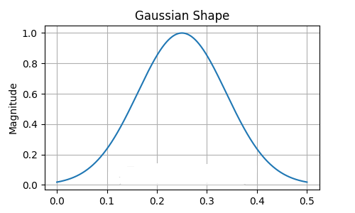
The gaussian function is the filter function favoured in this presentation.  Its shape tends to be more concentrated in the time domain. Indicating that it has a relatively shorter duration time compared to other filter functions. There are many trade offs that need to be considered when selecting an appropriate filter function. Here application requirements take precedence.

Filter specification

Filters encountered in this article are all specified by two parameters. The center frequency and the width parameter. Sometimes called the scale. Both should be given in terms of frequency cycles per sample. The center frequency can take on values in the range of 0 to 0.5. The width parameter determines the range of frequencies, above and below the center frequency, in the passband that will be passed through the filter function relatively unchanged. The width should take on values of about 0.01 and above.

In-phase filters

We begin our exploration of filter types with in-phase filters. The position of a waveform in time is called its phase. In-phase filters maintain the phase relationship of the input signal with the output. It means when an input signal passes through an in-phase filter, the filtered output will retain the same temporal relations as the input within the allowed frequency range.

Bandpass filters are a type of in-phase filter that serves as a fundamental building block that many other filters can be constructed from. The filter allows a specific range of frequencies to pass through while attenuating or rejecting frequencies outside this range. It operates by reducing signals with frequencies lower or higher than the passband.

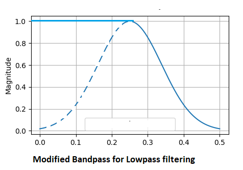
Lowpass and highpass filters are implemented by modifying the bandpass filter. A lowpass filter emphasizes low frequencies in a signal. Mostly used to detect the general tendency of a process. The lower the center frequency the smoother the filtered output will be. Using the bandpass filter function, we multiply all frequencies  less than or equal to the center frequency with the constant 1.0 and attenuate all others above, accordingly. 

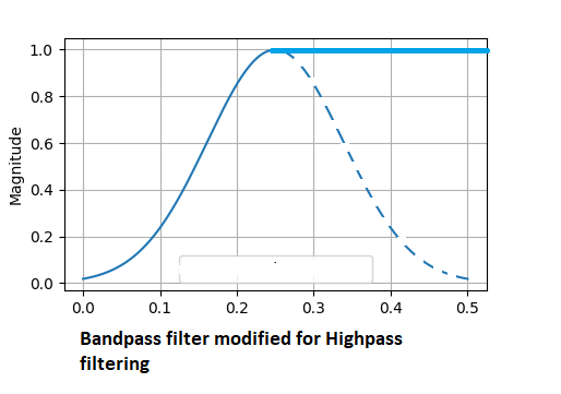
A highpass filter removes all slow variation from the signal leaving only information about rapid changes. In this case, all frequencies below the center frequency's lower passband are reduced. Leaving only frequencies in the higher bands to pass through.

There are numerous variations of in-phase filters, some of which may be better than those described so far. Those mentioned here all share the primary property of having adequately round filter shapes, which is an important quality that can not be emphasized enough.  

In-quadrature filters

These filters (also referred to as quadrature filters) are designed to process signals by applying a phase shift of 90 degrees (Pi/2 radians) relative to the input. They are only occasionally useful in solitude, and more commonly used in combination with in-phase filters. In certain situations, they are useful in detecting phase relationships within time series.

To understand the value of an in-quadrature filter, its best to observe an example. Below is a series depicted by a short periodic component.

The next plot is the bandpass filtered output of the series above. It highlights the in-phase nature of the bandpass filter. Movements in the filtered signal line up with those of the original series.

The following plot shows the filtered output from an in-quadrature version of the bandpass filter. Examining it closely it can be seen that peaks in the filtered signal correspond with zero crossings in the original signal. Basically, the in-quadrature filtered output, lines up with a shift applied to the in-phase bandpass output.

This implies that peaks in the in-quadrature output signal indicate a significant change in the input series. The peaks and troughs of an in-quadrature filter give an indication of fast changes occurring in the input signal. Alternatively, when the input signal is steady the output will be zero or nearer to zero. This means that in-quadrature filters are sensitive to changes that happen at certain rates.

Let's take a look at another example. The series below is characterized by a sharp abrupt move to the upside.

In-phase and in-quadrature filtered outputs of this series follow. Again, take note of the position of the peaks and troughs relative to the sharp move upwards. While it is difficult to ascertain the move using the in-phase output, the in-quadrature filtered series detects the explosive move.

The manner in which the two types of filters were used brings to light, their utility when used together. When an in-phase and in-quadrature filter with the same parameters are used together they are called a quadrature-mirror filter(QM filter).

Quadrature mirror filters

QM filters help in the detection of localized instances of periodic components. Using the QM filter we analyze the in-phase output relative to the in-quadrature output. Both of these outputs will be at zero when a particular periodic event is not present. The outputs from both can be combined by treating the in-phase output as the real part and the in-quadrature output as the imaginary part. Enabling the calculation of the amplitude and phase of the filtered waveform.

Before we look at the implementation of the code, we first have to deal with one of the most important aspects of any time series analysis procedure.

Preprocessing the series before transformation

The fact that time series are finite in length presents problems when converting them into the frequency domain with the DFT.  The DFT assumes the raw series is periodic and therefore repeats indefinitely. Applying the DFT to a non-periodic signal can induce distortions in the output's waveform.

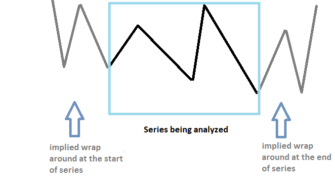
To mitigate the wrap around effects we have to taper the end of the series with extra constant values. Artificially increasing the number of samples in the series, can provide a finer frequency resolution and reduce spectral leakage. This is an operation referred to as padding. The padded series is converted using the DFT. The extra values added to the series help reduce distortions in the spectrum of the series, but these are not the only benefits.

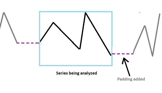
Increasing the length of the series so that the total number of samples is a power of 2, greatly aids the computational efficiency of the FFT algorithm. At first, it seems odd that deliberately increasing the length leads to better performance, but is true. So padding is essential. Besides using zeros, a series can be padded with the calculated mean value of the series.

Financial time series usually have the nasty habit of being non-stationary. When a series is padded, and the series contains a slow varying component. The sharp contrast in values at either end of the original series and the values used for padding can manifest as a prominent frequency component in the frequency domain. Causing contamination.

To guard against this form of distortion, the original series values have to be detrended. So the original series values are replaced with the detrended values. When we need to get back to the original time domain of the series, we just have to retrend the series. This will be demonstrated when we go over the implementation of the code in the next section.

The CFilter class

The CFilter class encapsulates basic examples of the three filter types discussed. The code is contained in Filter.mqh, which begins by including the fasttransforms.mqh from the ALGLIB library.

//+------------------------------------------------------------------+
//|  CFilter - class implementing select filters in the freq domain  |
//+------------------------------------------------------------------+
class CFilter
  {
   int               m_length;                   //length of original series
   int               m_padded_len;                //modified length of series
   int               m_half_padded_len;           //half of modded series
   double            m_slope, m_intercept;     //slope and intercept of trend in series
   double            m_buffer[];               //general internal buffer
   bool              m_initialized;              //initialization flag
   complex           m_dft[];                 //general complex buffer

public:
                     CFilter(double &series[],uint min_padding=0, bool detrend=true);
                    ~CFilter(void);

   void              Lowpass(double freq,double width,double &out[],bool add_trend);
   void              Highpass(double freq,double width, double &out[]);
   void              Bandpass(double freq,double width, double &out[]);
   void              Qmf(double freq,double width, complex &out[]);
   bool              IsInitialized(void) { return m_initialized; }
  };

CFilter has a parametric constructor, to which a user must pass the raw series to be filtered, as well as two other parameters that specify, the amount of padding to be applied and whether the series should be detrended before applying a DFT transformation. If zero is set for "min_padding", then the actual amount of padding will be only be determined by the number of samples. "min_padding" determines the minimum number of values that will be added to the series excluding any extra values included to lengthen the series to the nearest power of two.

Inside the constructor, after all arguments are checked, the final length of the padded series is calculated and detrending is applied if specified. The padded series is written to "m_buffer" array. And the DFT is applied with the waveform of the series given in "m_dft", an array of complex numbers. If any error is encountered in the constructor, "m_initialized" will be set to false.

//+------------------------------------------------------------------+
//|constructor                                                       |
//+------------------------------------------------------------------+
CFilter::CFilter(double &series[],uint min_padding=0,bool detrend=true)
  {
//---local variables
   m_initialized=false;
   int i;
   int npts = ArraySize(series);
   int pad = (int)MathAbs(min_padding);
//--- check size of series
   if(npts<=0)
     {
      Print("Input array is empty");
      return ;
     }
//---
   m_length = npts ;
   for(m_padded_len=2 ; m_padded_len<INT_MAX ; m_padded_len*=2)
     {
      if(m_padded_len >= npts+pad)
         break ;
     }
//---
   if(m_padded_len<npts+pad)
     {
      Print("Warning, calculated length of modified series is too long");
      return;
     }
//---
   m_half_padded_len = m_padded_len / 2;
//---
   ArrayResize(m_buffer,m_padded_len);
//---
   if(m_padded_len > npts)            // Any padding needed?
     {

      if(detrend)
        {
         m_intercept = series[0] ;
         m_slope = (series[npts-1] - series[0]) / (npts-1) ;
        }
      else
        {
         m_intercept = m_slope = 0.0 ;
         for(i=0 ; i<npts ; i++)
            m_intercept += series[i] ;
         m_intercept /= npts ;
        }

      for(i=0 ; i<npts ; i++)
        {
         m_buffer[i]=series[i] - m_intercept - m_slope * i ;
        }
      for(i=npts ; i<m_padded_len ; i++)
        {
         m_buffer[i]=0.0;
        }
     }

   else
     {
      ArrayCopy(m_buffer,series);
      m_intercept = m_slope = 0.0 ;
     }
//---Compute the Fourier transform of the padded series
   CFastFourierTransform::FFTR1D(m_buffer,int(m_padded_len),m_dft);
//---
   m_initialized = true;

  }

Users should check if an instance has been correctly constructed by calling "IsInitialized()". It should return true on success.

After successful instantiation, users can call any of the publicly accessible methods that applies a specified filter on the signal stored in "m_dft". Most of these have similar input requirements. First are the filter specifications, defined by the "freq" and "width" parameters. They correspond to the center frequency and width of the passband to be applied. Almost all the methods expect at least one last input array, where the results of the filtering operation will be saved.

"Lowpass()" is the only method that accepts a fourth input parameter which determines whether any detrending initially applied to the original signal should be reversed on the filter's output.

//+--------------------------------------------------------------------+
//|Filters series in frequency domain and returns output in time domain|
//+--------------------------------------------------------------------+
void CFilter::Lowpass(double freq,double width,double &out[],bool add_trend)
  {
//---
   int i ;
   double f, dist, wt ;
   complex dft_temp[];
   ArrayCopy(dft_temp,m_dft);
//---
   for(i=0 ; i<=m_half_padded_len ; i++)
     {
      f = (double) i / (double) m_padded_len ;  // This frequency
      if(f <= freq)                  // Flat to here
         wt = 1.0 ;
      else
        {
         dist = (f - freq) / width ;
         wt = exp(-dist * dist) ;
        }
      dft_temp[i].real*=wt;
      dft_temp[i].imag*=wt;
     }
//---
   double temp[];
//---
   CFastFourierTransform::FFTR1DInv(dft_temp,m_padded_len,temp);
//---
   ArrayResize(out, m_length);
//---
   for(int i = 0; i<m_length; i++)
      out[i]=(add_trend)?temp[i] + m_intercept + m_slope*i:temp[i];

  }

 There are two steps involved in the implementation of in-phase filters: First the waveform of the signal placed in "m_dft" is multiplied with the modified filter function. Which in this implementation is the Gaussian function. Finally an inverse DFT is conducted, returning the series to the time domain.  

To calculate the QM filter outputs, we multiply the DFT terms of a waveform with the in-quadrature version of a filter function. The in-quadrature filter function is simply an in-phase filter function with a phase shift of 90 degrees applied. To achieve this phase shift the in-phase filter function is multiplied by i, making it pure imaginary. The result is a function whose outputs are symmetric about the Nyquist frequency. The output terms on either side of the 0.5 frequency will be equal in absolute terms but opposite in sign.

The "Qmf()" method takes advantage of this fact by multiplying the DFT terms of the waveform with the sum of the in-phase and in-quadrature filter functions. This is done by making the in-quadrature filter function pure real,  ( recall that the in-quadrature filter function is pure imaginary) by multiplying it by i. When the filter functions are added together, outputs beyond the Nyquist frequency cancel each other out. In the code, the filtered DFT terms above 0.5 are set to 0. Only filtered outputs below and equal to the Nyquist frequency need to be calculated. Once the waveform has been filtered a complex inverse DFT is done to return to the time domain.

//+------------------------------------------------------------------+
//| Implements Quadrature Mirror Filter, output is complex           |
//+------------------------------------------------------------------+
void CFilter::Qmf(double freq,double width,complex &out[])
  {
//---
   int i ;
   double f, dist, wt ;
   complex dft_temp[];
   ArrayCopy(dft_temp,m_dft);
//---
   for(i=1 ; i<m_half_padded_len ; i++)
     {
      f = (double) i / (double) m_padded_len ;    // This frequency
      dist = (f - freq) / width ;
      wt = exp(-dist * dist) ;
      dft_temp[i].real *= wt ;
      dft_temp[i].imag *= wt ;
      dft_temp[m_padded_len-i].real = dft_temp[m_padded_len-i].imag = 0.0 ;  // Causes QMF outputs
     }

//---
   dft_temp[0].real = 0.0 ;
   dist = (0.5 - freq) / width ;
   dft_temp[m_half_padded_len].real = 0.5 * dft_temp[m_half_padded_len].imag * exp(-dist * dist) ;
//---
   dft_temp[0].imag = dft_temp[m_half_padded_len].imag = 0.0 ;     // By definition of real transform
//---
   CFastFourierTransform::FFTC1DInv(dft_temp,m_padded_len);
   ArrayResize(out,m_length);
//---
   for(i=0 ; i<m_length ; i++)
     {
      out[i].real = dft_temp[i].real/double(m_half_padded_len) ;
      out[i].imag = dft_temp[i].imag/double(m_half_padded_len) ;
     }
  }
//+------------------------------------------------------------------+

The AFD program

To demonstrate the use of CFilter we introduce AFD.mq5. An application implemented as  an expert advisor. It enables users to generate random sequences of a specified length. Users are able to set the length of the series to be generated and also adjust the seed of the random numbers used. The series is plotted in blue in the upper graph. Users can observe the result of applying a selected filter to the generated series, in the second plot. All parameters of the filter can be adjusted from the program's graphical user interface. The application is shown below.

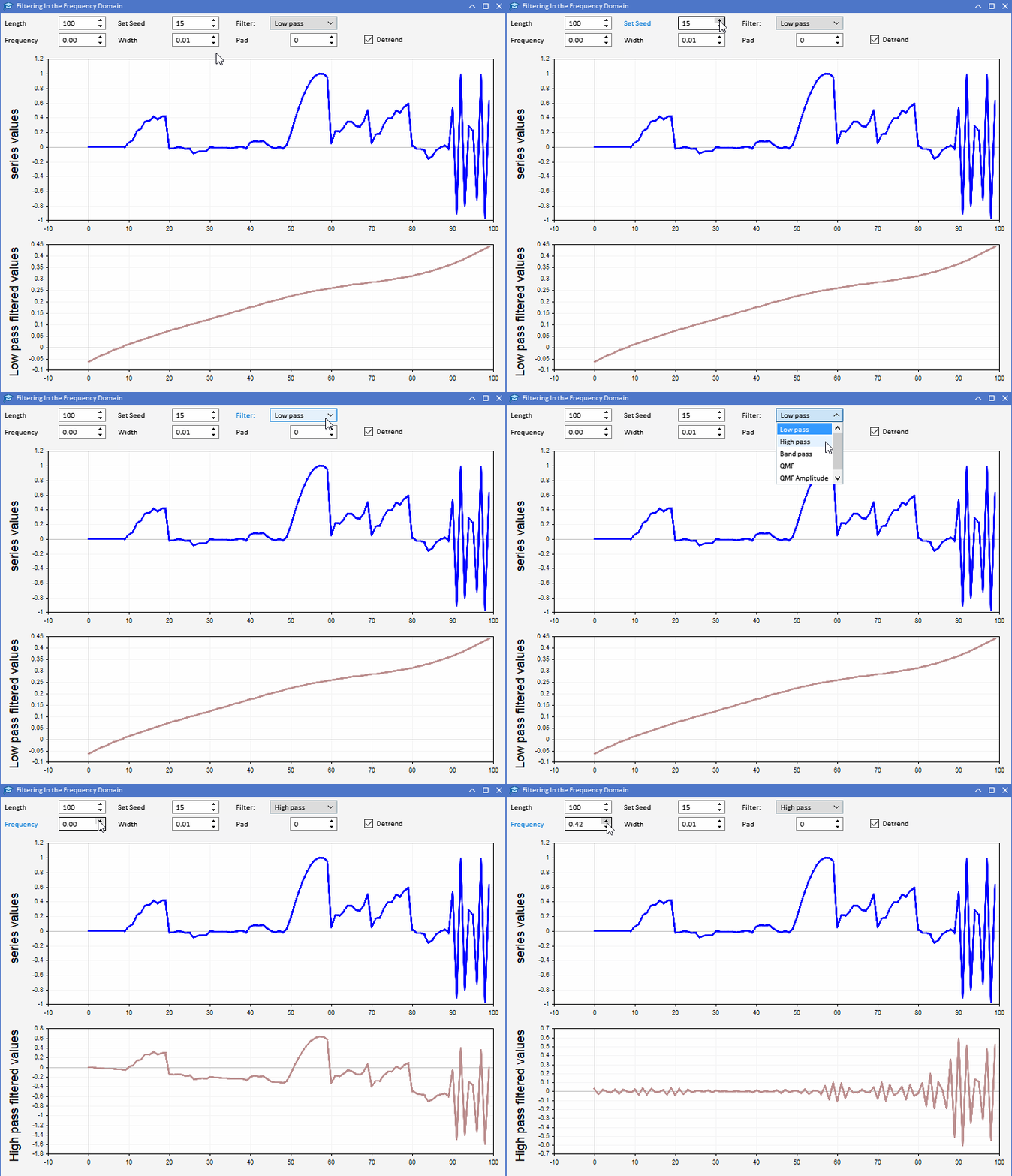
Using the AFD application we can develop a more intuitive appreciation of the different types of information revealed by filter outputs. The output from in-phase filters can be used in a number of two ways. Output from a lowpass filter can be used to supply information about the average value of the input series at any given time. Highpass filter output reveals the occasional highs and lows apparent in the original series. These outputs give a sense of the state of the input series at each time point.

Bandpass filter outputs are less obvious in terms of their relevance. It's probably impossible for anyone to make sense of the filter output through observation alone. Though it's possible that this data may be useful to a prediction model. Maybe knowing that the bandpass output for a particular passband is at a peak or trough signifies something in the original series.

Let's look at the bandpass output of a random series at different frequencies.

The outputs reveal another type of information. The peaks of the bandpass outputs portray the amount of periodic variation at a particular time slot. More precisely it  shows the amplitude of the variation, indicating the presence of periodic variation. Lower peaks signal lower variation and higher peaks the opposite.

The amplitude is given by sampling the QM filter output. Amplitude and phase calculations using QM filter values are shown in the code snippet below taken from AFD.mq5.

 case ENUM_QMF_AMPLITUDE:
        {
         y_name = "Amplitude";
         complex comp[];
         filter.Qmf(freq,scale,comp);
         ArrayResize(m_output1,ArraySize(comp));
         for(int i=0; i<ArraySize(m_output); i++)
            m_output1[i]=MathSqrt(comp[i].real*comp[i].real + comp[i].imag*comp[i].imag);
        }
      break;
      case ENUM_QMF_PHASE:
        {
         y_name = "Phase";
         complex comp[];
         filter.Qmf(freq,scale,comp);
         ArrayResize(m_output1,ArraySize(comp));
         for(int i=0; i<ArraySize(m_output); i++)
            m_output1[i]=(comp[i].real>=1.e-40 || comp[i].imag>=1.e-40)?atan2(comp[i].imag, comp[i].real):0.0;
        }
      break;

The difference in the bandpass output at different frequencies shows that there is a diversity of information available. It is therefore possible to construct unique features to supply to a machine learning algorithm. To construct these data sets intelligently a practitioner needs to have a solid grasp of the parameters that define a particular filter.

The width parameter

As mentioned earlier in the article, the parameters of all filters implemented are expressed in terms of frequency cycles per unit of time. One of the disadvantages of conducting analysis in the frequency domain is the difficulty in relating frequency components to their extent in the time domain. Using the example of the random series just viewed in the last section, the bandpass outputs were sampled at frequencies of 0.15, 0.3 and 0.45 all at the same width of 0.03. It's important to understand what these values mean, particularly in relation to the time domain of the series.

A frequency of 0.15 has a period of 1/0.15 = 6.67 samples per cycle. The width determines the resolution in the frequency domain. If we want to isolate a narrow frequency band, we apply a small width, 0.01 is usually the minimum, though it's possible to go lower. Again back to the example. The width was set to 0.03, so the passband stretches from 0.15-0.03 to 0.15+0.03 ie 0.12 to 0.18. Frequencies in this range will be passed through, with those above and below almost completely stopped.

The width also gives an indication of resolution in the time domain. The relationship between frequency domain resolution and time domain resolution is inverse. A higher resolution in one domain leads to a loss of resolution in another domain. To estimate  the time domain extent in relation to width we apply the following formula: 0.8/width

Using it we can estimate the number of samples in the time domain affected by the frequency passband relative to the current position. In other words, it estimates the number of samples before and after the current position that will have an effect on the observed output. Back to the example, a width of 0.03 implies a time extent of 0.8/0.03 = 27 samples. That means the value at each of the outputs is determined or influenced by 27 observations that came before and another 27 that comes after.

Generally speaking, the width of a filter should be proportional to the centre frequency of a passband we wish to study. This is related to the period of the frequency. Lower frequencies have longer periods whilst higher frequencies have shorter periods. Therefore for lower frequencies, we can afford to sacrifice resolution in the time domain and opt for a narrow width. Whereas higher frequencies benefit from broader width parameters, which translates to a shorter extent in the time domain.

Finally, the width parameter also has an effect on the values supplied to a prediction model.  Using the previous example whose implied time domain we calculated to be about 27 observations. Suppose we wanted to predict the next value of the series, at time slot number 201. We would supply the value of the filtered output, calculated based on the 200 known values, that is 27 slots from the end of the series. We cannot knowingly use any of the filtered output beyond this point because we know it would be subject to wrap around effects induced by the DFT, under the constraints of the filter's parameters.

In the last example we sampled filtered outputs at different frequencies but all at the same width. In practice it would be more beneficial to sample filtered outputs at strategically selected frequencies and widths so as to capture as much useful information as possible.

Conclusion

In summary, we have looked at three types of filters:

• In-phase filters help to break up a noisy series into different components highlighting important information and getting rid of distracting superfluous characteristics. By supplying relevant information to learning algorithms we can build better prediction models.

• In-quadrature filters can be used to detect regions of rapid level changes in a series. Although it may be easy to eyeball significant movements in a series, it can be difficult to convey such phenomena to a learning algorithm. This is the value of in-quadrature filters.

• The combination of both in-phase and in-quadrature filters work together to identify the presence of a periodic feature. These tools can be effective at identifying and studying features that manifest in a seemingly random manner in a time series.

Filtering in the frequency domain leverages the computational efficiency provided by the FFT algorithm. When compared to the method of convolution in the time domain, it's no contest. But, it's not all roses. Transformation of series to the frequency domain is fraught with pitfalls, that can result in totally bogus conclusions due to distortions introduced by careless data handling. So practitioners should be vigilant.

The code for all tools and programs is attached. The AFD.mq5 utilizes the venerable Easy and Fast (EAF) GUI library. It is available at mql5.com's code base. Just a side note, when using the EAF library along with ALGLIB, always make sure to include EAF last in your application, there are some naming conflicts between these libraries that hinder successful compilation.  

File Name	Description
Mql5\Include\Filter.mqh	Contains definition of CFilter class that implements basic digital filters in the frequency domain
Mql5\Include\RandomStationarySeries.mqh	Contains routines (functions) for generating random series of various characteristics. Used in AFD.ex5 application
Mql5\Experts\AFD.mq5	This is the source code of AFD application, it uses the Easy and Fast GUI library, listed on mql5.com codebase
Mql5\Experts\AFD.ex5	The compiled AFD application, implemented as an Expert Advisor