Neural networks made easy (Part 40): Using Go-Explore on large amounts of data

Introduction

In the previous article "Neural networks made easy (Part 39): Go-Explore, a different approach to exploration", we familiarized ourselves with the Go-Explore algorithm and its ability to explore the environment. As you might remember, the algorithm includes 2 stages:

• Phase 1 — explore
  
• Phase 2 — training the policy using examples

In Phase 1, we used random action selection to obtain as complete a picture of the environment as possible. This approach allowed us to collect a sufficient database of examples to successfully train an agent on historical data in one calendar month. The model we built was able to find a strategy for making a profit on the training set.

But the time period of one calendar month is too short to summarize the data and build a strategy that can make a profit in the foreseeable future. Consequently, to find our strategy, we are forced to increase the training period. When we extended the training period to three months, we found out that using random action selection did not result in a single profitable pass.

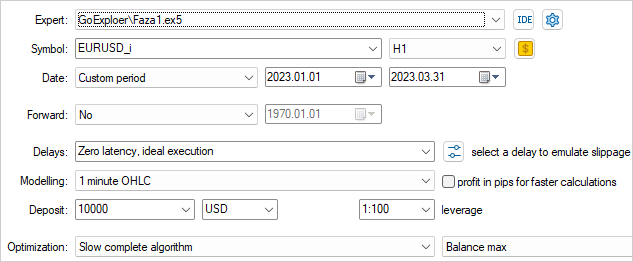
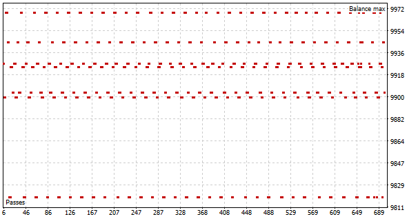
According to the probability theory, this is a completely expected result. After all, the probability of a total event is equal to the product of the probabilities of all its components. But since the probability of each individual event is less than 1, as the number of steps increases, the probability of obtaining a profitable pass decreases.

Besides, as the training period increases, there may be changes in the environment that may affect the agent's learning results. Therefore, it is important to regularly monitor the agent's performance and analyze its performance at intermediate stages.

To improve training results over a longer period, various optimization methods for the Go-Explore algorithm can be applied, for example, using an improved approach to action selection. This approach should take into account the broader context of the task and allow the agent to make more informed decisions.

In this article, we will take a closer look at possible optimization methods for the Go-Explore algorithm to improve its efficiency over longer training periods.

1. Difficulties in using Go-Explore as the training period increases

As the training period of the Go-Explore algorithm increases, certain difficulties arise. Some of them include:

1. Curse of dimensionality: As the training period increases, the number of states an agent can visit grows exponentially, making it more difficult to find the optimal strategy.

2. Environmental change: As the training period increases, changes in the environment may occur that may affect the agent's learning outcomes. This can cause a previously successful strategy to become ineffective or even impossible.

3. Difficulty in selecting actions: As the training period increases, the agent may need to consider the broader context of the task to make informed decisions. This can complicate the task of choosing the optimal action and require more complex methods for optimizing the algorithm.

4. Increased training time: As the training period increases, the time required to collect enough data and train the model also increases. This can reduce the efficiency and speed of agent training.

As the training period increases, the problem of increasing the dimension of the state space that needs to be explored may arise. This may lead to the "curse of dimensionality" problem, where the number of possible states grows exponentially with increasing dimensionality. This makes state space exploration difficult and can cause the algorithm to spend too much time exploring irrelevant states.

To solve this problem, dimensionality reduction techniques can be used, for example PCA. They allow reducing the dimensionality of the state space while maintaining information about the data structure. We can also use important feature selection techniques to reduce the dimensionality of the state space and focus on the most relevant aspects of the problem.

Besides, we can use additional methods such as optimization based on evolutionary or genetic algorithms, which allow us to search for optimal solutions in large state spaces. These methods allow us to explore various options for agent behavior and select the most optimal solutions for a given task.

Various approaches to action selection can also be used, such as confidence-based exploration methods, which allow the agent to explore new regions of state space, taking into account not only the probability of receiving a reward, but also the confidence in its knowledge about the task. This can help avoid the problem of getting stuck in local optima and allow for more efficient exploration of state space.

Reinforcement learning (RL) demonstrations typically use computer games or other artificially simulated environments that are stationary, meaning they do not change over time. However, in real-world applications, the environment may change over time, which may affect the agent's learning outcomes.

When using the Go-Explore algorithm, which includes an environmental exploration step to obtain historical data, changes in the environment can lead to unexpected results when the agent is subsequently trained on historical data.

For example, if the agent has been trained on data for several months and during this time there were changes in the environment, such as changes in the the game rules or the appearance of new objects, then the agent may not cope with the new environment, and its previously successful strategy may become ineffective or even impossible.

To reduce the impact of environmental changes on the agent's training results, it is necessary to regularly monitor the environment and analyze its changes throughout the agent's training. If significant changes in the environment are detected, it is necessary to restart the agent training process using updated data and algorithms.

We can also use training methods that take into account changes in the environment during training, such as model-based reinforcement learning (RL) methods, which build a model of the environment and use it to predict future states and rewards. This allows the agent to adapt to changes in the environment and make more informed decisions.

Other optimization techniques can be used, such as changing the hyperparameters of the algorithm or making changes to the algorithm itself to train more efficiently.

In general, using the Go-Explore algorithm to train agents over longer time periods can be quite complex and requires many technical solutions and improvements.

As a result, using the Go-Explore algorithm can be quite complex and requires many technical solutions and improvements. The Go-Explore algorithm is a powerful tool for exploring complex environments and training agents in tasks with a large number of states and actions. But its effectiveness may decrease with increasing training period and changing task conditions. Therefore, it is necessary to use various optimization methods and parameter tuning to achieve the best results. This could be a very useful and promising direction for research.

2. Options for optimizing the approach

Considering what was said above, extending the training period requires a more careful approach than simply specifying new dates in the strategy tester and loading additional historical data. To create a real trading strategy, it is necessary to train the model on as much historical data as possible. Only this approach will allow us to create a model capable of generating profit in the future.

In this article, we will not complicate the model. Instead, we will use several simple approaches that will help expand the depth of historical data for model training using the Go-Explore algorithm.

Before optimizing a previously created algorithm, it is necessary to analyze its bottlenecks.

The first step is to change the constants in the Cell structure. This structure is used to store a separate state of the system and the path that has been taken. Due to technical reasons, we are forced to use only static arrays in this structure. As the model training period increases, the size of the path to achieve the described state also increases. We have already created a constant indicating the size of the array. Now we should change the value of this constant so that there is enough space to record the entire path of the agent from the beginning to the end of the training period.

To determine the value of the constant, we will use simple math. On average, one calendar month contains 21-22 working days. To avoid errors, we will use the maximum value of working days - 22. There will be 88 working days in 4 months.

When testing models, we will use the H1 timeframe. There are 24 hours in a day. Thus, to train the model we will need a buffer of 2112 elements (88 * 24). These calculations take into account possible maximum values and slightly exceed the actual number of bars, which allows us not to be afraid of a critical error of exceeding the array size. However, when training on quotes including weekends (for example, cryptocurrency), calendar days should be used to calculate the buffer size, taking into account the full training period and the characteristics of the instrument quotes.

#define                    Buffer_Size  2112

The second bottleneck is sorting examples before saving them. Practice has shown that sorting data can take more time than going through historical data and collecting these states. As the training period increases, the amount of data for sorting will also increase. Therefore, we decided to abandon data sorting. As a result, the OnTesterDeinit function in the Faza1.mq5 advisor received the following form:

//+------------------------------------------------------------------+
//| TesterDeinit function                                            |
//+------------------------------------------------------------------+
void OnTesterDeinit()
  {
//---
   int total = ArraySize(Total);
   printf("total %d", total);
   Print("Saving...");
   SaveTotalBase();
   Print("Saved");
  }

During testing, it was discovered that the EA often opens several positions and keeps them open for a long time. We wanted to address this issue by taking a holistic approach and made several changes to how the sample collection EA works.

One of the changes relates to defining the remuneration. Previously, we used the change in equity as a reward. This approach allowed the model to take into account changes in accumulated and unrecorded profits, penalizing drawdowns and encouraging the accumulation of profits on profitable positions. However, this approach limited the possibilities of taking profit. We did not want to give up the benefit of using equity, but we also wanted to add a profit-taking reward.

We found a compromise solution that involved using the arithmetic average of the change in equity and account balance. When a profit or loss accumulates on an open position, the equity changes, but the account balance remains unchanged. The agent receives a reward or penalty equal to half the change in equity. When a profit or loss is recorded, the equity does not change, but the accumulated amount is reflected on the account balance. The agent receives the other half of the pending reward or penalty. Thus, the agent becomes more interested in closing positions with a profit and is less inclined to hold open positions.

      Base[action_count - 1].value = ( Base[action_count - 1].state[241] - state[241] + 
                                       Base[action_count - 1].state[240] - state[240] ) / 2.0f;

We also decided to limit the maximum volume of open positions to reduce their number. When creating examples and testing the model, we used a fixed minimum volume for each trade. Therefore, introducing a limit on the volume of open positions is completely identical to limiting the number of open positions. However, when describing the current state of the system, we collect information about the volume of open positions and accumulated profits/losses. To avoid additional calculations, we use the open position volume to limit the maximum volume. We moved the value of the maximum possible volume of an open position into external variables, which allows us to conduct experiments with different values.

input double               MaxPosition = 0.1;

The ultimate goal of our limiting the maximum volume of open positions is to reduce the number of open positions in the account and avoid the accumulation of trades in a positive or negative lock. To do this, we check the limit for long and short trades separately, without taking into account their difference.

It is important to note that we do not explicitly specify the constraints of our model. Instead, we apply restrictions on the maximum volume of open positions at the stage of creating examples that will be used to train the model. Next, we use these examples to train the model, and it itself builds its strategy based on the received examples. This approach allows the model to adapt to changing market situations and select the most effective actions.

However, it is worth considering that in the case when we generate an action to open a position, but due to the imposed restrictions it cannot be executed, the subsequent state of the system and the reward will not correspond to the generated action. To solve this problem, we save an action corresponding to the expectation (no trading) in the example database in case the generated action was not executed. This ensures the correspondence between action and reward and ensures that the model is trained correctly.

   switch(act)
     {
      case 0:
         if(buy_value >= MaxPosition || !Trade.Buy(Symb.LotsMin(), Symb.Name()))
            act = 3;
         break;
      case 1:
         if(sell_value >= MaxPosition || !Trade.Sell(Symb.LotsMin(), Symb.Name()))
            act = 3;
         break;
      case 2:
         for(int i = PositionsTotal() - 1; i >= 0; i--)
            if(PositionGetSymbol(i) == Symb.Name())
               if(!Trade.PositionClose(PositionGetInteger(POSITION_IDENTIFIER)))
                 {
                  act = 3;
                  break;
                 }
         break;
     }

Since we operate in conditions of risky market transactions, our task is not only to earn profits, but also to minimize possible losses. To do this, we add to our model a limit on the maximum time an open position can be held.

This limitation is an integer external variable that specifies the maximum number of bars to hold an open position. 

input int                  MaxLifeTime = 48;

We determine the lifetime of the oldest position and, when the boundary value is reached, we forcefully create an action to close all positions.

This is necessary so that we do not overhold open positions, which can lead to large losses. When collecting information about the current account status and open positions, we consider this limitation so as not to exceed the maximum holding time.

   int total = PositionsTotal();
   datetime time_current = TimeCurrent();
   int first_order = 0;
   for(int i = 0; i < total; i++)
     {
      if(PositionGetSymbol(i) != Symb.Name())
         continue;
      switch((int)PositionGetInteger(POSITION_TYPE))
        {
         case POSITION_TYPE_BUY:
            buy_value += PositionGetDouble(POSITION_VOLUME);
            buy_profit += PositionGetDouble(POSITION_PROFIT);
            break;
         case POSITION_TYPE_SELL:
            sell_value += PositionGetDouble(POSITION_VOLUME);
            sell_profit += PositionGetDouble(POSITION_PROFIT);
            break;
        }
      first_order = MathMax((int)(PositionGetInteger(POSITION_TIME) - time_current) / PeriodSeconds(TimeFrame), first_order);
     }

However, if we allow this limit to be exceeded, then appropriate measures should be taken. In this case, we do not simply close one position after time has expired, but specify the action to close all positions and close them all. This allows us to maintain a correspondence between the completed action, the new state and the reward, which is important for the correct operation of the model.

   int act = (first_order < MaxLifeTime ? SampleAction(4) : 2);

Thus, the use of a maximum time limit for holding an open position is another mechanism in our model that helps us control risks and achieve more stable results in case of uncertain market conditions.

We described approaches to optimizing the algorithm based on identified shortcomings during model testing. Now we move on to training the model on an expanded amount of historical data. Let's consider the possibility of splitting a large training set into smaller parts and training an agent in each of these parts. We can assume that if an algorithm works well over small time periods, then it can also work well over longer periods. Therefore, we can use this approach to improve model training on large amounts of data.

This approach allows the model to more effectively capture market trends and increases its resistance to changes in external factors. This is especially important when using the model to trade real markets, where predicting changes in trend direction is critical. In addition, this approach allows the model to more effectively use all available data, and not just the latest observations, which in turn improves the quality of forecasting.

It is important to note that dividing the training set into smaller time periods should be carried out taking into account the chronological order of the data in order to avoid data overlaps and biases in prediction. It is also necessary to take into account that when dividing the data into smaller segments, the amount of data available for training in each segment will be less, which can lead to a decrease in the prediction accuracy of the model.

Thus, splitting the training set into smaller time segments is an effective approach to optimizing the algorithm and can significantly improve the model's prediction quality.

When dividing the training set into smaller episodes, we are faced with the need to develop a general strategy that will allow us to successfully go through the entire training set. To do this, we can use a combination of random action sampling and directed step-by-step training, which will help us find the most successful and profitable strategy.

The idea is to play through small episodes sequentially, using a random sampling of actions in each episode. Then we select the most profitable passes and use them as a starting point for the next episode. Thus, we sequentially go through the entire training set, accumulating examples of a profitable strategy.

This approach combines seemingly opposing ideas: random sampling and directed training. Using random sampling, we explore the environment, and directed passage of the training sample helps us find the most successful strategy. As a result, we can get a more generalized and profitable strategy for our agent.

In general, combining random sampling and directed training allows us to obtain the most optimal strategy for passing the training sample, using both randomness and already accumulated experience of successful actions.

To implement this approach, we will introduce 3 external variables:

• MinStartSteps — minimum number of steps before sampling starts
• MaxSteps - maximum number of sampling steps (sequence size)
• MinProfit - minimum profit to save to the examples database.

input int                  MinStartSteps = 96;
input int                  MaxSteps = 120;
input double               MinProfit = 10;

While discussing algorithm optimization, we discovered that sorting examples before saving is inefficient. Instead, we decided to use the MinProfit variable to determine the minimum profit required for examples to be included in the database. This allows us to prioritize examples that are used as starting points for subsequent sampling. Additionally, we use the MinStartSteps variable to set the minimum number of steps in the example that is required to use it as a starting point. This allows us to avoid getting stuck in intermediate steps during the sampling process and move on to the next episode.

We also use the MaxSteps variable, which determines the maximum episode length. Once this value is exceeded, sampling is no longer effective and we need to save the path traveled. This way we can use resources more efficiently and speed up training.

In the OnInit method of the Faza1.mq5 EA, after loading the previously created database of examples, we first select examples that satisfy the requirement for the number of steps completed.

   if(LoadTotalBase())
     {
      int total = ArraySize(Total);
      Cell temp[];
      ArrayResize(temp, total);
      int count = 0;
      for(int i = 0; i < total; i++)
         if(Total[i].total_actions >= MinStartSteps)
           {
            temp[count] = Total[i];
            count++;
           }

After that, choose one example by random sampling out of the selected ones. It is this randomly selected example that we will use as the starting sampling point.

      if(count > 0)
        {
         count = (int)(((double)(MathRand() * MathRand()) / MathPow(32768.0, 2.0)) * (count - 1));
         StartCell = temp[count];
        }
      else
        {
         count = (int)(((double)(MathRand() * MathRand()) / MathPow(32768.0, 2.0)) * (total - 1));
         StartCell = Total[count];
        }
     }

In our EA's OnTick method, we first unconditionally execute the entire path until we reach the starting point of our episode.

void OnTick()
  {
//---
   if(!IsNewBar())
      return;
   bar++;
   if(bar < StartCell.total_actions)
     {
      switch(StartCell.actions[bar])
        {
         case 0:
            Trade.Buy(Symb.LotsMin(), Symb.Name());
            break;
         case 1:
            Trade.Sell(Symb.LotsMin(), Symb.Name());
            break;
         case 2:
            for(int i = PositionsTotal() - 1; i >= 0; i--)
               if(PositionGetSymbol(i) == Symb.Name())
                  Trade.PositionClose(PositionGetInteger(POSITION_IDENTIFIER));
            break;
        }
      return;
     }

We move on to action sampling operations only after reaching the beginning of our episode. At the same time, we control the number of random actions performed. Their number should not exceed the maximum episode length.

If the maximum number of steps is reached, we first generate an action to close all positions.

   int act = (action_count < MaxSteps || first_order < MaxLifeTime ? SampleAction(4) : 2);

After one move, we initiate the end of the EA’s work.

   if(action_count > MaxSteps)
      ExpertRemove();

After completing the passage in the strategy tester, we check the size of the profit received as a result of the pass. If the condition of reaching the minimum profitability threshold is met, we transfer the data to be added to the example database.

//+------------------------------------------------------------------+
//| Tester function                                                  |
//+------------------------------------------------------------------+
double OnTester()
  {
//---
   double ret = 0.0;
//---
   double profit = TesterStatistics(STAT_PROFIT);
   action_count--;
   if(profit >= MinProfit)
      FrameAdd(MQLInfoString(MQL_PROGRAM_NAME), action_count, profit, Base);
//---
   return(ret);
  }

Here we provide and explain only minor changes to the EA code, which was described in detail in the previous article. The full EA code can be found in the attachment.

3. Test

As in the previous article, we will collect examples for training the model using historical data on EURUSD H1. However, this time we will use historical data for 4 months of 2023.

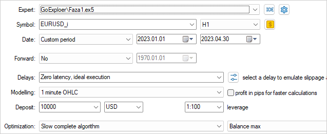
In order to most effectively explore the environment, it is necessary to use a variety of external parameter values during the sample collection. In this case, we will use these parameters as optimized ones, which will allow us to change their values for each pass.

To begin the optimization process, we will select two parameters: MaxSteps and MaxLifeTime. The first parameter determines the maximum length of an episode, after which collecting examples becomes ineffective. The second parameter indicates the maximum period for holding a position in one episode. By using different values of these parameters in the process of collecting examples, we can study the environment as fully as possible.

For example, by using different MaxSteps and MaxLifeTime values, we can collect examples for different durations and periods of position holding. This will allow us to obtain examples for a wide range of situations that may arise in the environment. In this way, we can create a more universal and effective training model that will take into account many different scenarios.

We set the threshold profit value close to 0. After all, this is the first pass and we only need to make a small profit.

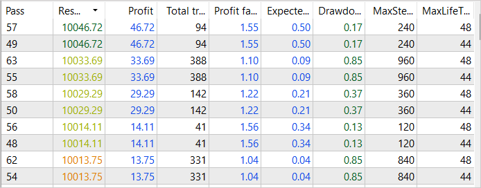
As a result of the first pass of the optimization process, we see several successful passes reaching a profit of USD 46 in the first 2 weeks of January 2023. The profit factor of such passes reaches 1.55

Before running the optimization, we will make some changes to the parameters. To ensure that examples are collected at different time intervals, we will add a minimum number of steps to our optimized variable before sampling begins. The values for this variable will vary from 1 to 3 weeks in weekly increments. In addition, we will improve the results obtained by increasing the profit threshold to USD 40.

Based on the results of the second optimization pass, we see an increase in profit to USD 84 for January 2023. Although there is a decrease in the profit factor to 1.38.

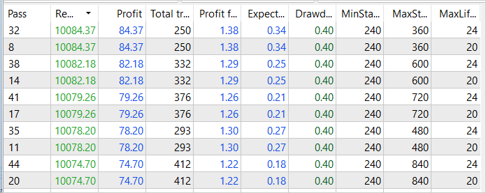
Despite this, we see that our efforts to optimize the sample collection process are beginning to bear fruit. Although we have not yet achieved final success, the general trend of events is consistent with our goals and expectations. 

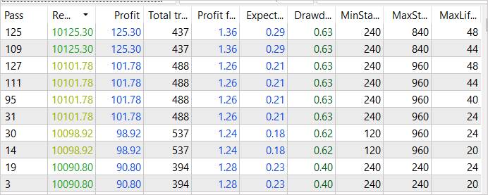
Let's increase the minimum number of steps before sampling starts in the second week of January 2023 and carry out another optimization process. This time we will increase the minimum profitability to USD 80. After all, we strive to find the most profitable strategy.

As we expected, we achieved even higher profitability as a result of subsequent optimization of the example collection process. The total income of the most successful pass has increased to USD 125. At the same time, the profit factor decreased slightly and amounted to 1.36, which still means that profits exceed costs. It is important to note that this increase in profitability was achieved through improvements in the sample collection process, and we can be confident in its efficiency. However, keep in mind that training is not yet complete, and we will continue it.

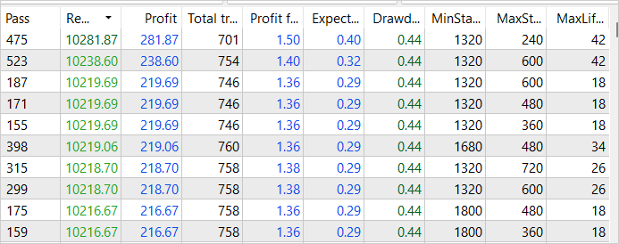
We continued iterations of collecting examples in the optimization mode of the strategy tester, successively shifting the starting point of sampling and changing the profit threshold. This approach allowed us to obtain examples of several successful passes through the entire training set. The most profitable of them yielded USD 281 in income with a profit factor of 1.5. These results confirm that our strategy for optimizing the case collection process has a positive effect and helps achieve higher profit margins. However, we understand that this process is not complete and requires further optimization and improvement.

Once the process of collecting examples is complete, we move on to training the model using the Go-Explore algorithm based on the data obtained. We then retrain the model using reinforcement training methods to further improve its performance.

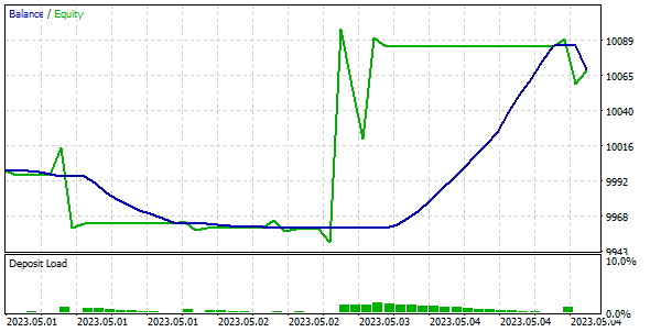
To check the quality and efficiency of the trained model, we test it on training and test samples. It is important to note that our model was able to make a profit on historical data for the first week of May 2023, which was not included in the training set but directly followed it.

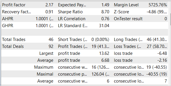
Conclusion

In this article, we looked at simple but effective methods for optimizing the Go-Explore algorithm, which allow it to be used for training models on large amounts of training data. Our model was trained on 4 months of historical data, but thanks to the use of optimization methods, the Go-Explore algorithm can be used to train models over longer time periods. We also tested the model on training and test samples, which confirmed its high efficiency and quality.

Overall, the Go-Explore algorithm opens up new possibilities for training models on big data and can become a powerful tool for various applications in the field of artificial intelligence.

However, it is important to remember that financial markets are very dynamic and subject to sudden changes, so even the best-quality model cannot guarantee 100% success. Therefore, we must constantly monitor changes in the market and adapt our model accordingly.

Links

1. Go-Explore: a New Approach for Hard-Exploration Problems
2. Neural networks made easy (Part 35): Intrinsic Curiosity Module
3. Neural networks made easy (Part 36): Relational Reinforcement Learning
4. Neural networks made easy (Part 37): Sparse Attention
5. Neural networks made easy (Part 38): Self-Supervised Exploration via Disagreement
6. Neural networks made easy (Part 39): Go-Explore, a different approach to exploration

Programs used in the article

#	Name	Type	Description
1	Faza1.mq5	Expert Advisor	First phase EA
2	Faza2.mql5	Expert Advisor	Second phase EA
3	GE-lerning.mq5	Expert Advisor	Policy fine tuning EA
4	Cell.mqh	Class library	System state description structure
5	FQF.mqh	Class library	Class library for arranging the work of a fully parameterized model
6	NeuroNet.mqh	Class library	A library of classes for creating a neural network
7	NeuroNet.cl	Code Base	OpenCL program code library