Category Theory in MQL5 (Part 22): A different look at Moving Averages

Introduction

Category Theory’s application to Finance has been the mainstay of articles in these series. We have dwelt a lot on time series forecasting because it is pertinent to most traders and they are the majority of members on this platform. However other relevant applications outside of this do include valuation, risk, portfolio allocation and many others. And perhaps to do a quick rundown on a valuation example, there is a plethora of ways in which category theory could be applied in obtaining the valuation of a stock. For instance, if we take the key stock metrics to each be an object in a category, then the morphisms (or graph paths) linking across these different metrics (like revenues, debt, etc.) can be attributed to different valuation classes (say A+, A, B, etc.). With this, once we have a particular stock’s metrics, we can then quantify by how much it belongs to a particular class. This is a simplified approach that is only meant to serve as a hint to what could be done within this purview.

Sticking to time series though, moving averages though overlooked by some as being too simplistic, are very significant in technical analysis primarily because their concept is foundational to so many other indicators e.g. Bollinger Bands, MACD, etc. They could be thought of as a less volatile view of price action, and emphasis on the ‘less-volatile’ is important given the amount of white noise in the markets.

For this article we will continue with the theme on natural transformations we introduced in the last article by exploring the ability of natural transformations to bridge the gap between related data sets of different dimensions. ‘Dimensions’ here is used to represent column count within a data set. So as before we are faced with two categories, one of a ‘simple’ series of raw prices, and the other with a ‘compound’ series of moving average prices. Our purpose will be to show applications in time series forecasting with a scope of only three functors.

Background

So, to begin let’s review some basic definitions of what we are considering here. A functor is a function mapping two categories. We will be dealing with three here and these can be thought of as composed in the diagram below:

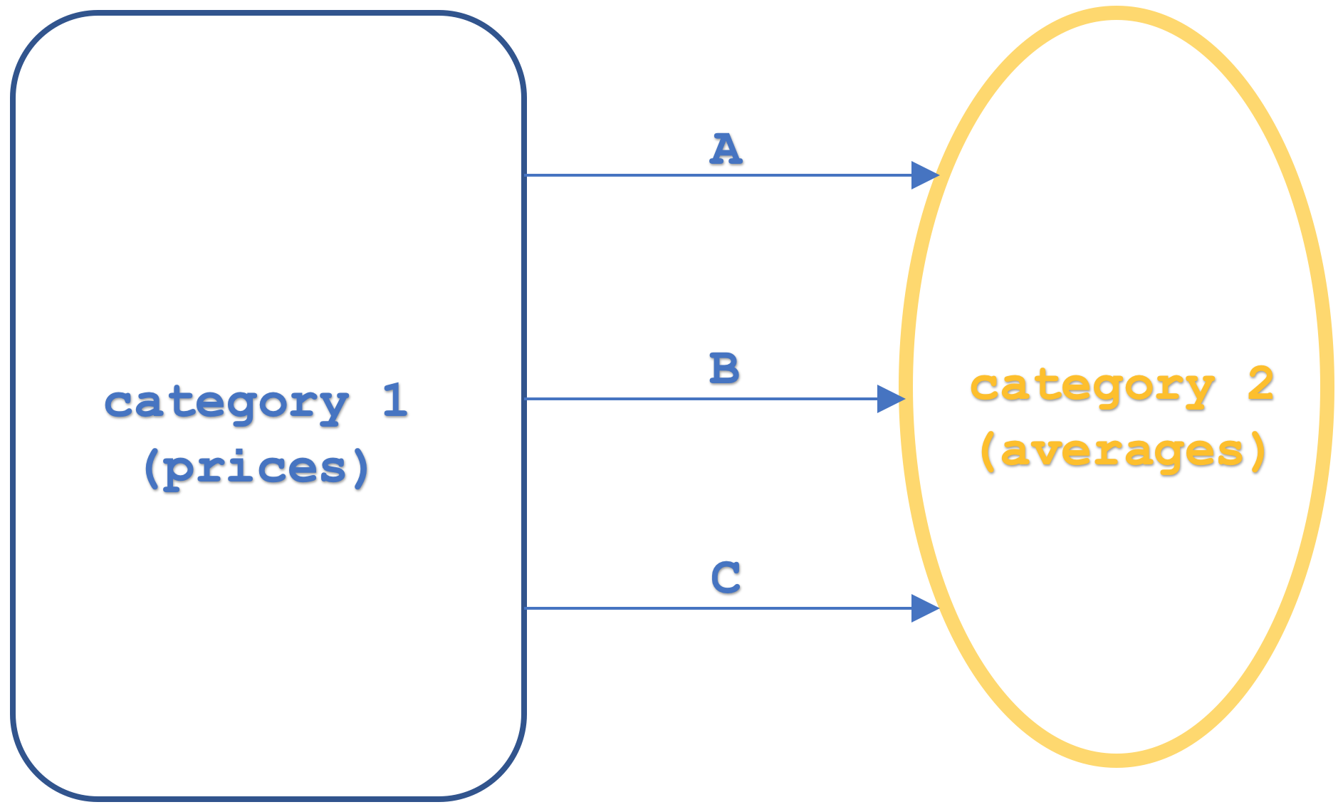
Our domain category has objects with price values at set time intervals, while the codomain objects of moving average price values also at similar time intervals. We have three functors highlighted namely A, B, and C. We have represented functors linking categories in recent articles what is new here is the addition of a third functor. This serves our purposes because it shows natural transformations in a ‘vertical’ arrangement. The ‘vertical’ setup is indicated on the diagram but in order to avoid any future ambiguity ‘vertical’ refers to natural transformations between functors that share the same domain and codomain category. This means if categories were diagrammatically positioned vertically and our natural transformations appeared to be pointing in the horizontal direction, the natural transformations would still be in a ‘vertical’ arrangement.

Moving on, moving averages are typically used as trading indicators by watching for their cross over points. These can be where they cross the underlying price such that a cross to the top is bearish as it represents a resistance barrier while a cross to the bottom is bullish since it indicates support. More often though these cross over points are between two moving averages of different periods. So typically, when the shorter period average crosses above the longer period we now have bullish setup since the longer and therefore less volatile moving average is indicating support while conversely if the shorter period average were to break below the longer it would be bearish. To that end this model has each functor representing a particular averaging period. So functor A will be the shortest of all three while functor B period will be in between and functor C will have the longest averaging period.

If we look at the categories we are considering, it may be helpful to outline why these two time-series meet the category axioms. To recap, we have already covered how orders (to which time-series are more relatable) can be construed as categories, nonetheless the axioms for a category are objects, morphisms, identity morphisms, and association. Both the domain and codomain categories are price time-series so illustrations with one is easily inferred in the other. If we therefore focus on the raw prices’ category (the domain), each price point is an object consisting two elements. Time and Price. The morphisms are the sequential mappings between the price points, since each price point follows another price point. The identity morphism at each price point can be thought of as a moving average at a period of one, this is the same as the price series but what the one period average provides is the identity relationship. Finally, composition with association is easily implied since given and three consecutive price points L, M, & N

L o (M o N) = (L o M) o N

The price after the morphism from M to N, when related to the morphism from L is the same as the price at N when related to the result of the morphism from L to M.

Categories and Functors

Our category 1 which will be the domain category for all functors will as mentioned feature a raw price time-series from which the functors map their averages.

This category will thus have in total 4 functors of which only 3 are of interest as far as we’re concerned. The first which is just worth a mention is the identity functor. This is because categories and functors behave pretty much like objects and morphisms, so identity needs to be present. The other three functors which as mentioned represent different moving average implementations will have each of their periods set by integer input parameters namely ‘m_functor_a’, ‘m_functor_b’, & ‘m_functor_c’ for the functors A, B, & C respectively.

The second category which constitutes the codomain to our three functors will have three objects each with moving average prices in a time series. So, each functor from the raw price series in category 1 will map to its own object in category 2.

Category 2 will have a lone origin functor which as mentioned would be the identity one. The morphisms between these objects would be equivalent to natural transformations as per the definitions we looked at in our last articles. This all could be summed up with the slightly more detailed diagram below:

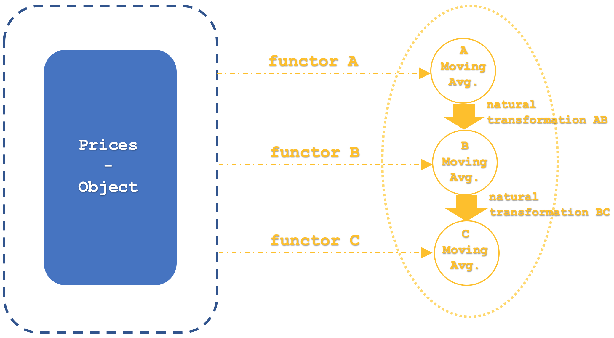
Our functor mapping for this article does not use third party algorithms like multi-layer perceptron, or random distribution forest, or linear discriminant analysis as we have in the recent articles. Rather it is the moving average algorithm, and the natural transformations will even be simpler as they will be the arithmetic difference between the end values of the two functors under consideration.

Natural Transformations

To define natural transformations in the context of Finance is like treading into no-man’s land. There is not a lot of material or references to back one up. What is often used or considered are other methods like correlation which has two major implementations; Pearson’s and Spearman. There are other methods that could be used for comparison but for this article we will use correlation of Spearman as part of our signal generation algorithm.

So, a natural transformation between two functors is the net difference of the target objects of the functors. In our case we have 3 functors which implies 3 possible natural transformations. We are though going to focus on just two transformations namely that between functor A & functor B which we can refer to as AB; and that between functor B & functor C which we will call BC. In using these two functors, we want to create two buffers of data for each. So, we will track the respective difference in moving averages and log them in their respective arrays thus creating two buffers of data. What we do with these buffers then is track their correlation coefficient. Tracking this value presents the thesis of our trade signal. A positive value should indicate the markets are trending, while a negative value does point to whipsaw markets.

Concretely therefore our signal will look to match the sum of all incremental changes in the moving averages with the indicated signal. So, if this value is positive than that indicates bullishness conversely if it is negative then that indicates bearishness. This signal which is bound to always produce a value on each bar will be filtered, as mentioned above, by the correlation between the two natural transformation buffers. Put differently our system asks whether there is any supplemental benefit in tracking natural transformations given that we already have established trends with each moving average.

Vertical Composition of Natural Transformations

Within category theory, the phrases "vertical composition" and its antithesis "horizontal composition" of natural transformations can occasionally have swapped meanings based on context and convention of the authors. It would not be strange to find some literature refer to natural transformations across functors that share domain and codomain categories as “horizontal compositions”. This is not the definition we will use. Just to be clear in this article and probably those that follow vertical composition will refer to natural transformations across functors that share domain and codomain categories.

So, what is the significance of vertical composition? From the conventions we’ve adopted, it is the simpler of the two. It provides a way of looking at two relatively simple data sets (which could be inferred as categories) and deriving special relationships across them that could easily be overlooked when dealing with multiple categories in more complex settings.

A good illustration of this should be our choice of a price series dataset and a moving average dataset for this article. But outside of trading another more insightful example could be in the culinary field. Consider a list of cooking ingredients (domain category) and a collection of menus (codomain category). Our functors would simply pair the ingredients to their respective menus. Natural transformations like functors and morphisms do preserve the definitions and structure of their origins. This may seem trivial but it is a corner stone concept in category theory. So, with the object’s elements and structure set (i.e. the menus and their items), natural transformations between the menus can help measure and assess the relative time it takes to prepare each dish or the cost of each dish, and a host of other areas of interest depending on a chef/ restaurant’s focus. Armed with this information, one can exploit isomorphism and explore deriving ingredients given a set of different menus. While this can be done with other methods and systems, category theory provides a structure preserving and quantifiable approach.

Forecasting Price Changes

Leveraging this vertical composition, in forecasting price changes is done by logging and analyzing the correlation coefficients of our two natural transformation buffers. These arrays need to be initialized since once the expert first starts running not enough data is loaded to perform a correlation. This is handled as shown in this listing:

//+------------------------------------------------------------------+
//| Get Direction function from Natural Transformations.             |
//+------------------------------------------------------------------+
void CSignalCT::Init(void)
   {
      if(!m_init)
      {
         m_close.Refresh(-1);
         
         int _x=StartIndex();
         
         m_o_prices.Cardinality(m_functor_c+m_functor_c);
         for(int i=0;i<m_functor_c+m_functor_c;i++)
         {
            m_e_price.Let();m_e_price.Cardinality(1);m_e_price.Set(0,m_close.GetData(_x+i));m_o_prices.Set(i,m_e_price);
         }
         
         m_o_average_a.Cardinality(m_transformations+1);
         m_o_average_b.Cardinality(m_transformations+1);
         m_o_average_c.Cardinality(m_transformations+1);
         
         for(int i=0;i<m_transformations+1;i++)
         {
            double _a=0.0;
            for(int ii=i;ii<m_functor_a+i;ii++)
            {
               _a+=m_close.GetData(_x+ii);
            }
            _a/=m_functor_a;
            m_e_price.Let();m_e_price.Cardinality(1);m_e_price.Set(0,_a);m_o_average_a.Set(i,m_e_price);
            //
            double _b=0.0;
            for(int ii=i;ii<m_functor_b+i;ii++)
            {
               _b+=m_close.GetData(_x+ii);
            }
            _b/=m_functor_b;
            m_e_price.Let();m_e_price.Cardinality(1);m_e_price.Set(0,_b);m_o_average_b.Set(i,m_e_price);
            //
            double _c=0.0;
            for(int ii=i;ii<m_functor_c+i;ii++)
            {
               _c+=m_close.GetData(_x+ii);
            }
            _c/=m_functor_c;
            m_e_price.Let();m_e_price.Cardinality(1);m_e_price.Set(0,_c);m_o_average_c.Set(i,m_e_price);
         }
         //
         ArrayResize(m_natural_transformations_ab,m_transformations);ArrayInitialize(m_natural_transformations_ab,0.0);
         ArrayResize(m_natural_transformations_bc,m_transformations);ArrayInitialize(m_natural_transformations_bc,0.0);
         
         for(int i=m_transformations-1;i>=0;i--)
         {
            double _a=0.0;
            m_e_price.Let();m_e_price.Cardinality(1);m_o_average_a.Get(i,m_e_price);m_e_price.Get(0,_a);
            double _b=0.0;
            m_e_price.Let();m_e_price.Cardinality(1);m_o_average_b.Get(i,m_e_price);m_e_price.Get(0,_b);
            double _c=0.0;
            m_e_price.Let();m_e_price.Cardinality(1);m_o_average_c.Get(i,m_e_price);m_e_price.Get(0,_c);
            
            m_natural_transformations_ab[i]=_a-_b;
            m_natural_transformations_bc[i]=_b-_c;
         }
         
         m_init=true;
      }
   }

We have declared three moving average handles for each functor and we need to refresh these before reading any values from them. Each moving average’s period is an input parameter so we have ‘m_functor_a’, ‘m_functor_b’, & ‘m_functor_c’, for the handles ‘m_ma_a’, ‘m_ma_b’, & ‘m_ma_c’ respectively. We also have two buffers for each natural transformation namely ‘m_natural_transformations_ab’, and ‘m_natural_transformations_bc’. The size of these arrays is set by the input parameter ‘m_transformations’ so at the onset both the arrays need to be resized to its value. The objects in the codomain category namely: ‘m_o_average_a’, ‘m_o_average_b’, and ‘m_o_average_c’, also need to be resized to this value plus one in order to be able to get all change increments.

So, the influence of different moving average periods on the ability to forecast, with this system, will be assessed if signals generated from matching changes in the moving average when the correlation of the natural transformation buffers is greater than zero. This is captured by the straight forward ‘GetDirection’ function listed below:

//+------------------------------------------------------------------+
//| Get Direction function from Natural Transformations.             |
//+------------------------------------------------------------------+
double CSignalCT::GetDirection()
   {
      double _r=0.0;
      
      Refresh();
      
      MathCorrelationSpearman(m_natural_transformations_ab,m_natural_transformations_bc,_r);
      
      return(_r);
   }

And each of the ‘CheckOpenLong’ and CheckOpenShort’ functions that compute our ‘trend’. This trend sets the signal direction with the ‘direction’ acting as a filter for whipsaw markets. Implementation of this is listed here:

      m_ma_a.Refresh(-1);
      m_ma_b.Refresh(-1);
      m_ma_c.Refresh(-1);
      
      int _x=StartIndex();
      
      double _trend= (m_ma_a.GetData(0,_x)-m_ma_a.GetData(0,_x+1))+
                     (m_ma_b.GetData(0,_x)-m_ma_b.GetData(0,_x+1))+
                     (m_ma_c.GetData(0,_x)-m_ma_c.GetData(0,_x+1));

We also need a function to refresh these values that is very similar to the ‘Init’ function. Full source code is attached at the end of the article.

On Back testing on the forex pair USDJPY from 1999.01.01 to 2020.01.01 on the daily time frame we get the report below with some of our ideal settings:

If we attempt to walk forward with these settings from 2020.01.01 to 2023.08.01, we do get the report below:

A positive walk is indicated which as always does not mean we have a working system but rather we could have something that can be tested on longer periods to confirm our early findings here.

Test Bed for Trade System Development

Integrating this signal class into a new or existing trade system can happen seamlessly thanks to the MQL5 wizard. All we have to do is assemble a new expert with this signal class as one of the other signals that a trader either always uses or wants to try out. The typical input parameter of ‘Signal_XXX_Weight’ (where XXX is the name of the signal class) whose value typically ranges from 0.0 to 1.0 can be optimized across all signals to determine the appropriate weight for each.

The evaluation of such a trading system should be on the merits of the trader’s needs. Usually it’s a see-saw between growth versus capital preservation. Back-of-the-envelope I would say AHPR is the best metric for growth while Recovery Factor would be for safety? This is all rough estimation so the reader and serious trader would need to undertake some more diligence in arriving at what works for them.

With a performance assessment system in place, next and perhaps equally important would be having a method of incrementally improving the strategy without compromising its premise and ability to walk-forward. With this there is no cut and dry method rather than constantly checking on back test and walk forward performance with each iteration or modification in the system.

There is also the possibility as always of having an instance of a trailing class that is based on this model. We would have to make a few changes but the overall gist would be the same. For starters our moving averages rather than using the close price as the applied price, would use something that leans towards volatility this could be the typical price or perhaps even better the median price. Secondly the forecast direction would still point to correlations between the two natural transformations buffers but in this case, we would track the current change in the bar range to act as our ‘trend’. So, decreases in the range would need to be backed by in positive correlations (values more than zero). The same would apply for increasing volatility. If the correlation is zero or negative then this would imply our model is indicating any current changes in volatility can be ignored. An implementation of this is also attached at the end of this article.

Conclusion

To summarize, the impact of natural transformations in a vertical composition is something that sounds too academic and archaic to draw any interest from most people. And yet it is arguably insightful because by looking at illustrations with common indicators, such as the moving average for this article, we have exposed a few patterns, from which we were able to read confirmation signals when forecasting a time series.

The use of this to develop a robust trade system is always where the rubber meets the road and requires a bit more work on the part of the trader to bring to fruition. None the less there is arguably enough support material online for the determined trader to see this through.

I urge further exploring of these concepts outside of time series forecasting and into other areas of trading and finance like valuation, or risk in order for readers to be more comfortable with what is shared here.

References

Citations for this article are mostly from Wikipedia.

Resources for Implementing the Category Theory Concepts in this article are attached below. They are the class file on category theory named ‘ct_22.mq5’, and the trailling file ‘TraillingCT_22_r1.mqh’. The class file should be put in the ‘include’ folder while the trailling file should be put in ‘Include\Expert\Trailling’ folder. Readers unfamiliar with the MQL5 wizard may want to refer to this article here on how to assemble expert advisors with the wizard because this signal file is meant to be used by assembling it in the wizard.