
MQL5 Wizard Techniques you should know (Part 19): Bayesian Inference
Introduction
We continue our exploit of MQL5 wizard by reviewing Bayesian inference, a method in statistics that processes and updates probabilities with each new information feed. It clearly has a broad spectrum of possible applications, however for our purpose as traders, we zero in on its role in forecasting time series. The time series open to traders for analysis are primarily prices of the traded securities, but as we’ll see in this article, these series could be ‘expanded’ to also consider alternatives like security trade history.
In theory, Bayesian Inference should enhance market-adaptability of any trade system, since the re-assessment of any hypothesis in inherent. This should lead to less curve fitting when tested on historical data and subsequently given forward walks or live account drills. But that is the theory and in practice implementation can wreck a sound idea, which is why we’ll try to consider more than one possible implementation of Bayesian Inference for this article.
Our article, thus, is structured in a simple format that covers the definition of Bayesian inference, application examples that cover illustrations in a custom signal class, money-management class, and trailing stop-class; strategy testing reports, and finally a conclusion.
Definition
Bayesian Inference (BI) is held up by the formula P(H|E) = [P(E|H) * P(H)] / P(E), where:
- H stands for the hypothesis, and
- E evidence, such that;
- P(H) is the prior probability of the hypothesis, while,
- P(E) is the evidence probability aka marginal likelihood.
- P(H|E) and P(E|H) are respective conditional probabilities of the above, and they are also referred to as posterior probability and likelihood respectively.
The above formula while simple and straight forward does present a bit of a chicken-and-egg problem namely how do we find: P(E|H). This is because it does imply from our listed formula above that its solution:
P(E|H) = [P(H|E) * P(E)] / P(H).
However, this could also be re-written as P(E|H) = [P(E∩H)] / P(H). Which would allow us to do some manual workarounds in this situation, as we’ll see below.
Signal Class
The signal class typically establishes the position an Expert Advisor should take, whether long or short. It does so by adding up indicator weightings, and the sum value always ranges from 0 to 100. In using BI, we are faced with a wide berth of time series choices, however this article, for the signal class, will only provide illustration with the close price change time series.
To use this time series, or any other type for that matter, we firstly need to find a ‘systematic’ way of either classifying the time series values or clustering them. This obvious step is important because it not only normalizes our time series data, it allows us to properly identify it when processing its probability.
Clustering is unsupervised, and we use a rudimentary approach of it, assigning a cluster to each data point depending on the type of price change. All positive values get assigned a cluster, zero values their own cluster and negative values also have their own. We have considered alternative clustering approaches in the past within these article series and the reader is welcome to experiment with these however for this article, seeing as clustering is not the prime subject, we have considered something very elementary.
Even with this basic clustering approach, it becomes clear that we can better ‘identify’ the data points and therefore assess their probabilities. Without it, since the data is floating point, each one would have been unique which in essence would amount to a unique cluster type and this clearly would defeat our purpose in getting and computing the probability values. Our simple approach is implemented in the source below:
//+------------------------------------------------------------------+
//| Function to assign cluster for each data point                   |
//+------------------------------------------------------------------+
void CSignalBAYES::SetCluster(matrix &Series)
{  for(int i = 0; i < int(Series.Rows()); i++)
   {  if(Series[i][0] < 0.0)
      {  Series[i][1] = 0.0;
      }
      else if(Series[i][0] == 0.0)
      {  Series[i][1] = 1.0;
      }
      else if(Series[i][0] > 0.0)
      {  Series[i][1] = 2.0;
      }
   }
}
Once we have the data points ‘identified’ we’d then proceed to work out the posterior probability as defined in the formula equation above. In doing so, though, we would need a specific cluster type that serves as our hypothesis. This cluster is bound to be unique for long positions and short positions, therefore we have custom input parameters for each that serve as indices that identify the type of cluster to use in each case. These are labelled ‘m_cluster_long’ and ‘m_cluster_short’ respectively.
So, to get the posterior probability, this cluster index together with the ‘identified’ or clustered time series would be required as inputs. Our function that calculates posterior probability is getting the probability of the position types’ cluster occurring given the current cluster type. Since we are providing a series of recent data points, each with its cluster index in a matrix format, we essentially have the zero-index data point as the current cluster.
In order to resolve our potential chicken-and-egg situation mentioned above we do work out as P(E|H).
From first principles. Since H is represented by the respective position index as explained above, the evidence E is the current cluster or the cluster type at index zero within the input series. So, our posterior probability is finding out the likelihood that a given position’s cluster type occurs next given that the latest evidence (cluster at index 0), has occurred.
Therefore, to find P(E|H) the reverse, we revisit the input series and do an enumeration of when the position index H occurred followed by the zero index E (the evidence). This also is a probability, so we would first enumerate the space i.e. find the H occurrences and then within that space find how many times the evidence index followed in succession.
This clearly implies that our input series is of sufficient length, subject to the number of cluster types under consideration. In our very simple example we have 3 cluster types (actually 2 considering the zero-price change is bound to seldom occur) and this could work with an input series of less than 50. However, should one opt for a more adventurous clustering approach were 5/6 or more types of clusters are used then the default size of the input series needs to be substantial enough to capture occurrence of all these cluster types for our posterior function to work. The listing for the posterior function is below:
//+------------------------------------------------------------------+
//| Function to calculate the posterior probability for each cluster |
//+------------------------------------------------------------------+
double CSignalBAYES::GetPosterior(int Type, matrix &Series)
{  double _eh_sum = 0.0, _eh = 0.0, _e = 0.0, _h = 0.0;
   for(int i = 0; i < int(Series.Rows()); i++)
   {  if(Type == Series[i][1])
      {  _h += 1.0;
         if(i != 0)
         {  _eh_sum += 1.0;
            if(Series[i][1] == Series[i - 1][1])
            {  _eh += 1.0;
            }
         }
      }
      if(i != 0 && Series[0][1] == Series[i][1])
      {  _e += 1.0;
      }
   }
   _h /= double(Series.Rows() - 1);
   _e /= double(Series.Rows() - 1);
   if(_eh_sum > 0.0)
   {  _eh /= _eh_sum;
   }
   double _posterior = 0.0;
   if(_e > 0.0)
   {  _posterior += ((_eh * _h) / _e);
   }
   return(_posterior);
}
Once we get our posterior probability, it would represent the likelihood of the position’s optimal cluster type (whether ‘m_cluster_long’ or ‘m_cluster_short’) occurring given the current cluster type (i.e. the evidence or the cluster type for the data point at index zero). This would be a value in the range 0.0 to 1.0. For the respective hypothesis whether for long or short positions, to be probable, the returned value ideally would have to be more than 0.5, however special situations could be explored by the reader where slightly lesser value could yield interesting results.
The decimal value though, would have to be normalized to the standard 0 – 100 range that is outputted by the long condition and short condition functions. To achieve this, we simply multiply it by 100.0. The typical listing of a long or short condition is listed below:
//+------------------------------------------------------------------+
//| "Voting" that price will grow.                                   |
//+------------------------------------------------------------------+
int CSignalBAYES::LongCondition(void)
{  int result = 0;
   vector _s_new, _s_old, _s;
   _s_new.CopyRates(m_symbol.Name(), m_period, 8, 0, m_series_size);
   _s_old.CopyRates(m_symbol.Name(), m_period, 8, 1, m_series_size);
   _s = _s_new - _s_old;
   matrix _series;
   _series.Init(_s.Size(), 2);
   for(int i = 0; i < int(_s.Size()); i++)
   {  _series[i][0] = _s[i];
   }
   SetCluster(_series);
   double _cond = GetPosterior(m_long_cluster, _series);
   _cond *= 100.0;
   //printf(__FUNCSIG__ + " cond: %.2f", _cond);
   //return(result);
   if(_cond > 50.0)
   {  result = int(2.0 * (_cond - 50.0));
   }
   return(result);
}
With this signal class it can easily be assembled in to any Expert Advisor via the MQL5 wizard by using guides that are here and here for readers that may be new to the MQL5 wizard.
Money Management Class
A custom money management (MM) class can be implemented as well that utilizes BI. Once again to start we would need to select an appropriate time series to base our analysis on, but as alluded to in the introduction our choice for this with MM will be historical trade performance. So, since our wizard assembled Expert Advisor will be trading just the one symbol all the trade history available for selection, on query, will be applicable to the Expert Advisor.
In utilizing trade history time series as a basis for the analysis, we’ll be taking a leaf from one of the inbuilt money management classes that is ‘size optimized’ where trade volume size is reduced in proportion to the recent number of consecutive losses. In our case, though, we’ll reduce the lot of size if the likelihood of our preferred cluster index (the hypothesis) falls below another optimizable parameter that we are calling ‘m_condition’.
So, what we are trying to establish in essence is the ideal cluster index at which we can use regular lot sizing in proportion to free margin. This cluster index is an identifier for the type of equity curve (since only one symbol is traded) at which we are free to scale lot size in proportion to free margin. The reference to ‘type of equity curve’ is a bit broad since our clustering follows the simple format we adopted in the signal class then what is being specifically pinpointed here is type of trade result i.e. whether win or loss (zero profit results are allocated an index but are unlikely to feature materially in the analysis).
This means for instance if the favourable trade result for scaling of lot size with free margin is a profitable trade result then we would be examining the sequence of previous trade results and trying to establish the likelihood of having another profitable trade result in light of the evidence (the trade result at the zero index of the input series).
This kind of necessitates another optimizable parameter in the form of a probability threshold that gauges the likelihood of repeating the target favourable conditions such that if the posterior result falls short of this threshold then position sizing is reduced in proportion to the number of losses counted as is the case in the original ‘optimized size’ money management class. The listing for the optimize function is below:
//+------------------------------------------------------------------+
//| Optimizing lot size for open.                                    |
//+------------------------------------------------------------------+
double CMoneyBAYES::Optimize(int Type, double lots)
{  double lot = lots;
//--- calculate number of losses orders without a break
   if(m_decrease_factor > 0)
   {  //--- select history for access
      HistorySelect(0, TimeCurrent());
      //---
      int       orders = HistoryDealsTotal(); // total history deals
      int       losses=0;                    // number of consequent losing orders
      //--
      int      size=0;
      matrix series;
      series.Init(fmin(m_series_size,orders), 2);
      series.Fill(0.0);
      //--
      CDealInfo deal;
      //---
      for(int i = orders - 1; i >= 0; i--)
      {  deal.Ticket(HistoryDealGetTicket(i));
         if(deal.Ticket() == 0)
         {  Print("CMoneySizeOptimized::Optimize: HistoryDealGetTicket failed, no trade history");
            break;
         }
         //--- check symbol
         if(deal.Symbol() != m_symbol.Name())
            continue;
         //--- check profit
         double profit = deal.Profit();
         //--
         series[size][0] = profit;
         size++;
         //--
         if(size >= m_series_size)
            break;
         if(profit<0.0)
            losses++;
      }
      //--
      series.Resize(size,2);
      SetCluster(series);
      double _cond = GetPosterior(Type, series);
      //--
      //---
      if(_cond < m_condition)
         lot = NormalizeDouble(lot - lot * losses / m_decrease_factor, 2);
   }
//--- normalize and check limits


...

//---

...

//---

...

//---
   return(lot);
}
All the other parameters of decrease factor and margin percentage invested remain the same as in the original ‘size optimized’ MM class.
For comparison to BI, we could consider the Kelly Criterion, which considers winning results and risk to reward ratio, but with a long term view and not necessarily updating allocation criteria through recent or intermediate performance. Its formula is given as K = W – ((1 - W) / R)
Where:
- K is percentage allocation
- W is winning percentage &
- R is the profit factor
This approach has reportedly been adopted by investment gurus because of its long-term outlook in allocating capital however it can be argued that it is positioning that ought to take a long-term approach not the allocation. Long-term outlooks are often adopted in matters of operation, however where risk is involved the short term tends to be more critical which is why execution is a separate subject.
So, the advantages of BI over the Kelly Criterion (KC) could be summed up with the argument that KC assumes a constant edge in the markets, which can be true in cases where one has a very long horizon. The ignoring of transaction costs & slippage is another similar argument against KC and while both could be ignored over the very long term it’s fair to say that the way most market are set up is to allow someone to trade on behalf of, or with someone else’s capital. This inherently implies that a fair degree of sensitivity needs to be applied to these short-term excursions, as they can determine whether the trader or investor is still entrusted with the capital in play.
Trailing Stop Class
Finally, we look at a custom trailing class implementation that also utilizes BI. Our time series for this will have to focus on price bar range as this is always a good proxy for volatility, a key metric in influencing by how much a stop loss level should be adjusted for open positions. We have been using changes in time series values as for signal we used changes in close price while for MM we used trade result (profits as opposed to account equity levels) which are also de-facto changes in account equity levels. Changes when applied to our rudimentary clustering method do give us a very basic but workable set of indices that are useful in grouping these floating-point data points.
A similar approach for an expert trailing class would focus on the changes in the high to low price bar range. Our hypothesis with this approach would be that we are looking for a cluster index (‘m_long_cluster’ or ‘m_short_cluster’ both could be the same in this situation of trailing) such that when it is more probable for it to follow in the time series, then we need to move our stop loss by an amount proportional to the current price bar range.
We have used separate input parameters for long and short positions, but in principle we could have used only one to serve both long and short position stop loss adjustment. Our listing implementing this is given below for long positions:
//+------------------------------------------------------------------+
//| Checking trailing stop and/or profit for long position.          |
//+------------------------------------------------------------------+
bool CTrailingBAYES::CheckTrailingStopLong(CPositionInfo *position,double &sl,double &tp)
  {
//--- check

...

//---

...

//---
   sl=EMPTY_VALUE;
   tp=EMPTY_VALUE;
   //

   vector _h_new, _h_old, _l_new, _l_old, _s;
   _h_new.CopyRates(m_symbol.Name(), m_period, COPY_RATES_HIGH, 0, m_series_size);
   _h_old.CopyRates(m_symbol.Name(), m_period, COPY_RATES_HIGH, 1, m_series_size);
   _l_new.CopyRates(m_symbol.Name(), m_period, COPY_RATES_LOW, 0, m_series_size);
   _l_old.CopyRates(m_symbol.Name(), m_period, COPY_RATES_LOW, 1, m_series_size);
   _s = (_h_new - _l_new) - (_h_old - _l_old);
   matrix _series;
   _series.Init(_s.Size(), 2);
   for(int i = 0; i < int(_s.Size()); i++)
   {  _series[i][0] = _s[i];
   }
   SetCluster(_series);
   double _cond = GetPosterior(m_long_cluster, _series);
   //
   delta=0.5*(_h_new[0] - _l_new[0]);
   if(_cond>0.5&&price-base>delta)
     {
      sl=price-delta;
     }
//---
   return(sl!=EMPTY_VALUE);
  }
A comparison of this with alternative trailing stop classes such as those inbuilt within the MQL5 library is provided in the testing and reports section below.
Testing and Reports
We perform tests on EUR JPY on the 4-hour time frame for the year 2022. Since we have developed 3 separate custom classes usable in wizard experts we will sequentially assemble 3 separate expert advisers with the first having only the signal class while money management utilizes fixed lots and no trailing stop is used; the second will have the same signal class but with the addition of the money management class we have coded above and no trailing stop; while the final Expert Advisor will have all 3 classes we coded above. Guidelines on assembling these classes via the wizard are available here.
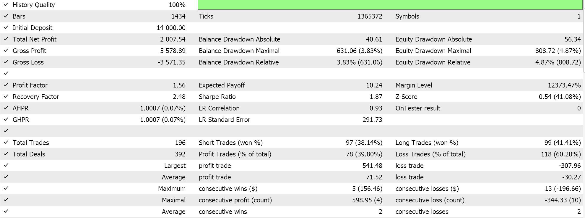
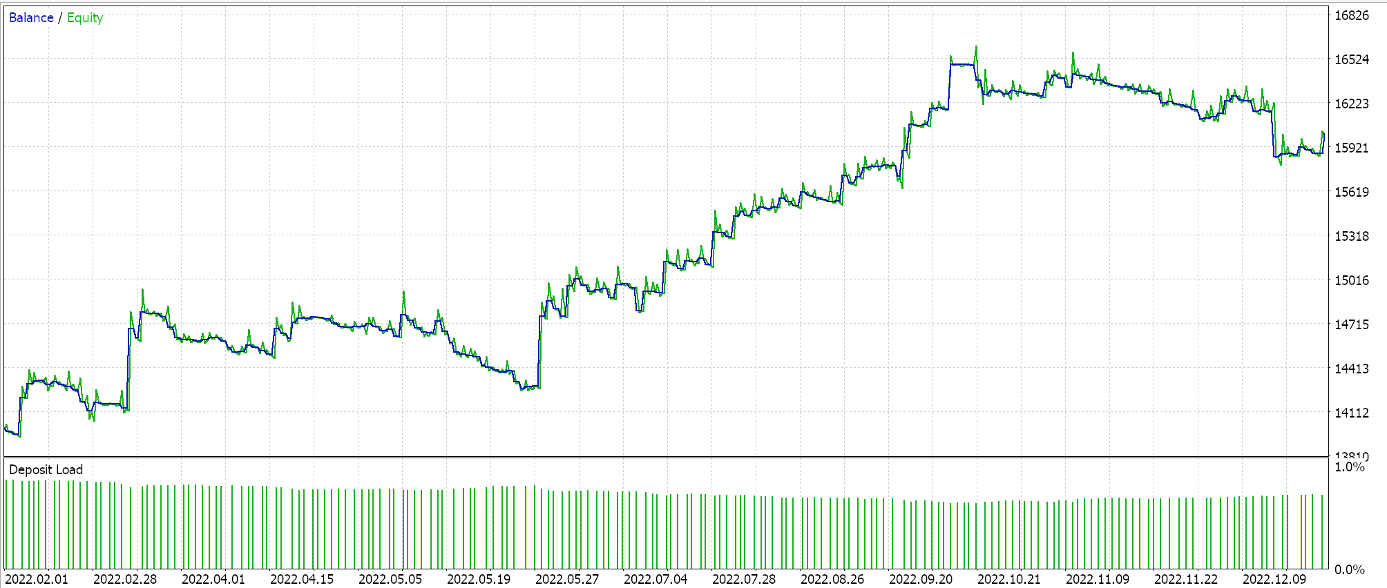
If we run tests on all three Expert Advisors, we get the following reports and equity curves:
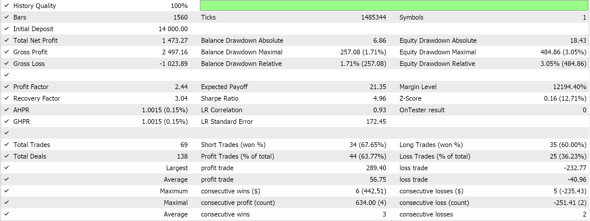
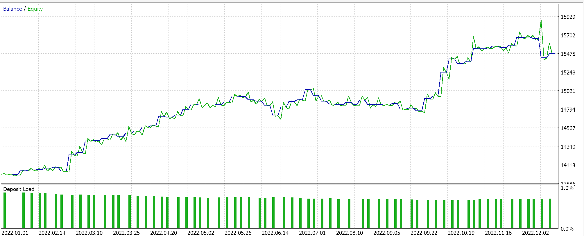
Report and equity curve of Expert Advisor with BI signal class only.
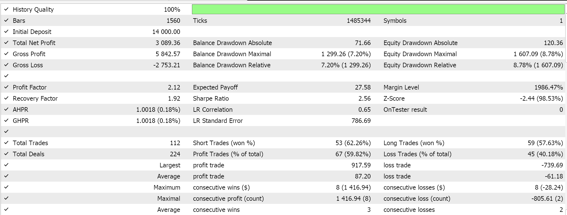
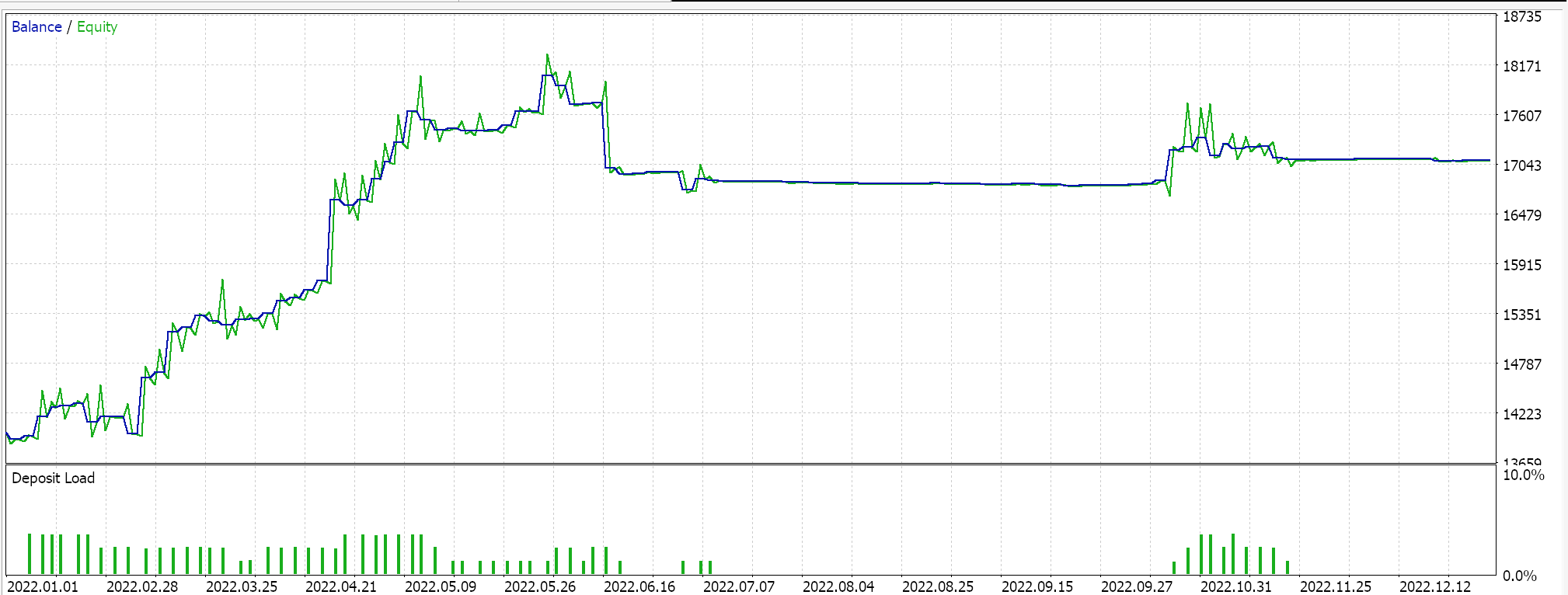
Report and equity curve of Expert Advisor with BI signal class and MM class only.
Report and equity curve of Expert Advisor with BI signal class, MM and trailing class.
It does appear that as more adaptation of BI from the signal class through MM to the trailing class is made, the overall performance does tend to correlate positively. This testing is done on real ticks, but as always independent testing over longer periods is ideal, and it is something the reader should keep in mind. As a control, we can optimize 3 separate Expert Advisors that use the library classes. In all these test runs, we do not use exit price targets and are only relying on the open and close signal to control the exits. We pick the awesome oscillator signal class, size optimized money management class and moving average trailing classes as what to use in the ‘control’ Expert Advisors. Similar test runs as above do yield the following results:
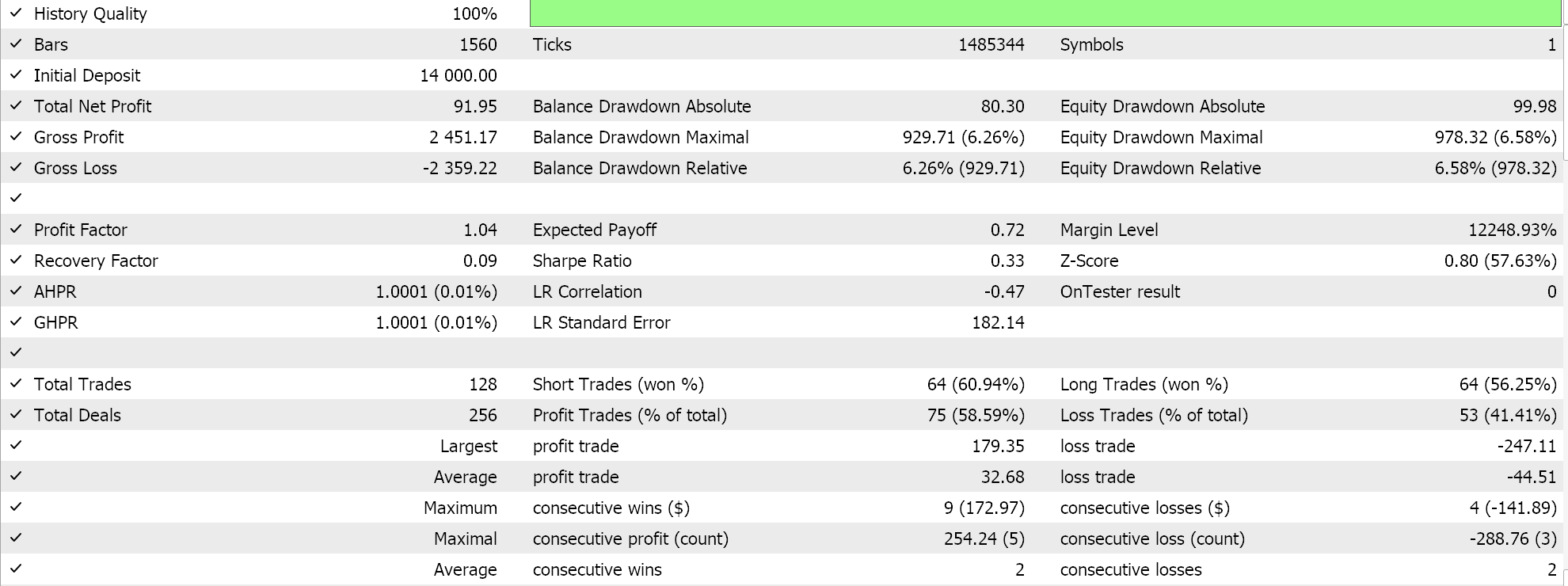
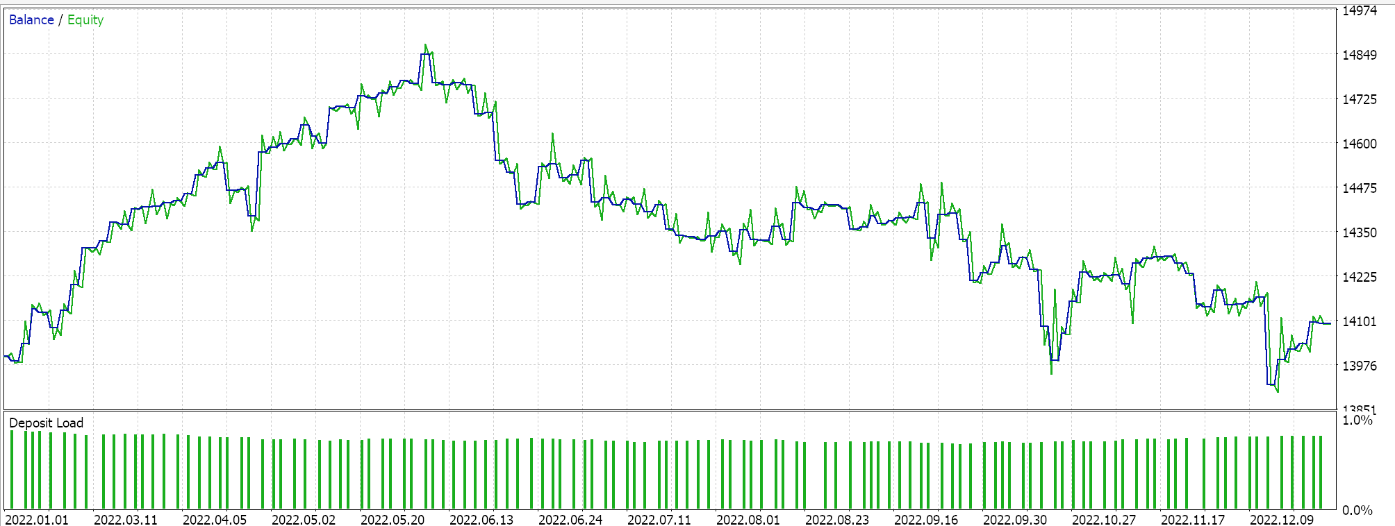
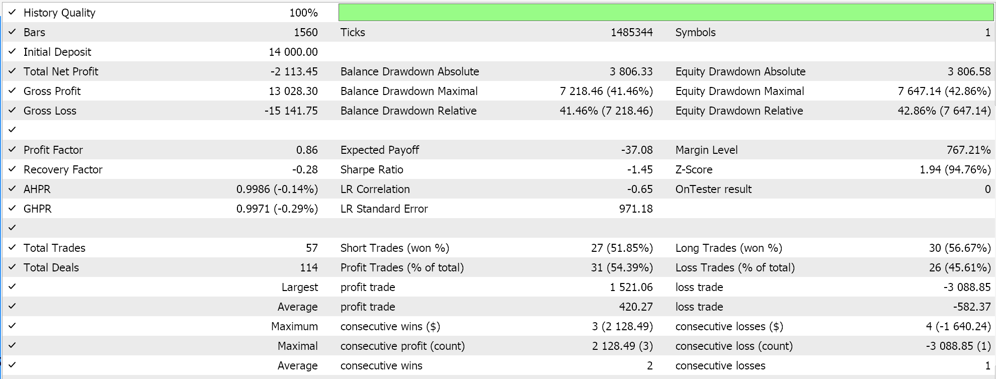
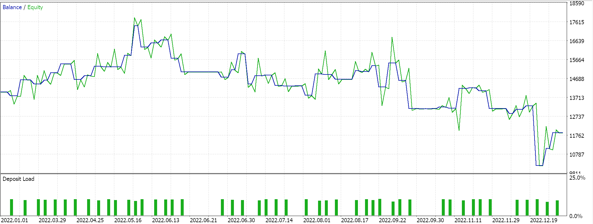
Report and equity curve of Expert Advisor with only the awesome oscillator class.
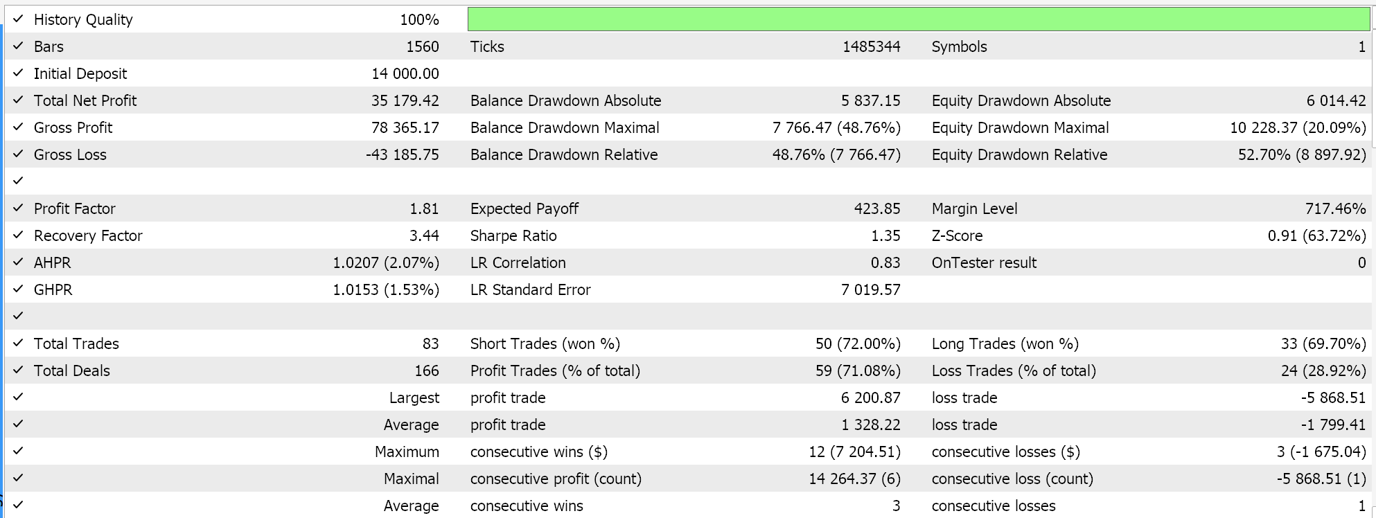
Report and equity curve of control Expert Advisor with 2 of the selected classes.
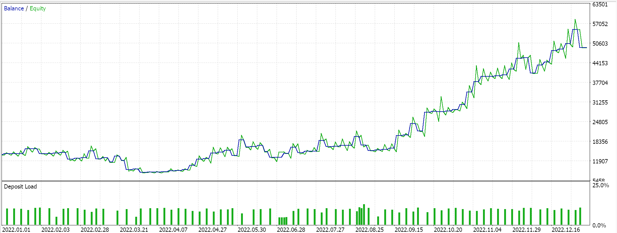
Report and equity curve of control Expert Advisor with all 3 selected classes.
The performance of our control does lag the BI expert, with the exception being in the third run. Our choice of alternative signal, MM and trailing classes did also sway this ‘result’ a lot, however the overall goal was to establish if there is significant variance in performance between our BI Expert Advisor and what is readily available from the MQL5 library and to that the answer is clear.
Conclusion
To conclude, we have tested Bayesian Inference’s role in building a simple Expert Advisor by incorporating its basic ideas in the three different pillar classes of MQL5 wizard assembled Expert Advisors. Our approach here was strictly introductory and did not cover significant ground, especially as this relates to using more elaborate cluster algorithms or even multi dimensioned data sets. These are all avenues that can be explored and could provide one with an edge if properly tested over decent history periods, on good quality tick data. A lot more can test under Bayesian Inference and the reader is welcomed to explore this as the wizard assembled experts remain a reliable tool in testing and prototyping ideas.
 Population optimization algorithms: Binary Genetic Algorithm (BGA). Part I
 Statistical Arbitrage with predictions
 Developing an MQL5 RL agent with RestAPI integration (Part 3): Creating automatic moves and test scripts in MQL5
 A feature selection algorithm using energy based learning in pure MQL5
- Free trading apps
- Over 8,000 signals for copying
- Economic news for exploring financial markets
You agree to website policy and terms of use