MQL5 中的矩阵和向量操作
MetaQuotes | 5 十二月, 2022
特殊数据类型 — 矩阵和向量 — 已被添加到 MQL5 语言中,以便解决一大类数学问题。 新类型提供了内置方法,能够创建接近数学标记符号的简洁易懂的代码。 在本文中,我们所提供的内置方法简介来自矩阵和矢量方法帮助部分。
内容
- 矩阵和向量类型
- 创建和安装
- 复制矩阵和数组
- 复制时间序列数据至矩阵和数组
- 矩阵和向量运算
- 操纵
- 乘积
- 变换
- 统计
- 特征
- 求解方程
- 机器学习方法
- 基于 OpenCL 的改进
- MQL5 在机器学习中的未来
每种编程语言都会提供数组数据类型,可存储数值变量集合,包括 int、double、和其它类型。 数组元素依据索引访问,能够利用循环进行数组操作。 最常用的是一维和二维数组:
int    a[50];       // One-dimensional array of 50 integers
double m[7][50];    // Two-dimensional array of 7 subarrays, each consisting of 50 integers
MyTime t[100];      // Array containing elements of MyTime type
数组的能力通常足以完成与数据存储,及处理相关的相对简单的任务。 但当涉及复杂的数学问题时,由于大量的嵌套循环,数组操作在编程和代码阅读两方面变得越发困难。 即使是最简单的线性代数运算,也需要繁复的编码,以及对数学的良好理解。
机器学习、神经网络、和 3D 图形、等现代数据技术广泛运用与向量和矩阵概念相关的线性代数解决方案。 为了灵活操作这类对象,MQL5 提供了特殊的数据类型:矩阵和向量。 新类型消减了许多常规编程操作,提高了代码质量。
矩阵和向量类型
简而言之,向量是一维的双精度型数组,而矩阵是二维的双精度型数组。 向量可以是垂直和水平的,然而,它们在 MQL5 中不分彼此。
矩阵可以表示为水平向量数组,其中第一个索引是行号,第二个索引是列号。
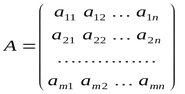
行和列编号从 0 开始,类似于数组。
除了包含双精度型数据的“矩阵”和“向量”类型之外,还有四种类型可用于相关数据类型的操作:
在撰写本文时,matrixc 和 vectorc 类型的工作尚未完工,故尚无法在内置方法中使用这些类型。
模板函数支持 matrix<double>、matrix<float>、vector<double>、vector<float> 等表示法,替代对应的类型。
  vectorf       v_f1= {0, 1, 2, 3,};
  vector<float> v_f2=v_f1;
  Print("v_f2 = ", v_f2);

  /*
  v_f2 = [0,1,2,3]
  */
创建和安装
矩阵和向量方法根据其用途划分为九大类。 有若干种方式能够声明和初始化矩阵和向量。
最简单的创建方法是不指定大小的声明,即不为数据分配内存。 在此,我们只编写数据类型和变量名:
  matrix         matrix_a;   // double type matrix
  matrix<double> matrix_a1;  // another way to declare a double matrix, suitable for use in templates
  matrix<float>  matrix_a3;  // float type matrix
  vector         vector_a;   // double type vector
  vector<double> vector_a1;  // another notation to create a double vector
  vector<float>  vector_a3;  // float type vector
然后,您可以更改创建对象的大小,并用所需的数值填充它们。 它们还可用在内置矩阵方法中,由此获得计算结果。
矩阵或向量可以按指定的大小声明,同时分配内存,但数据不会初始化。 于此,在变量名称之后,在括号中指定大小:
  matrix         matrix_a(128,128);           // the parameters can be either constants
  matrix<double> matrix_a1(InpRows,InpCols);  // or variables
  matrix<float>  matrix_a3(InpRows,1);        // analogue of a vertical vector
  vector         vector_a(256);
  vector<double> vector_a1(InpSize);
  vector<float>  vector_a3(InpSize+16);       // expression can be used as a parameter
创建对象的第三种方式是声明并进行初始化。 在这种情况下,矩阵和向量大小由大括号中指示的初始化数字序列确定:
  matrix         matrix_a={{0.1,0.2,0.3},{0.4,0.5,0.6}};
  matrix<double> matrix_a1=matrix_a;                      // the matrices must be of the same type
  matrix<float>  matrix_a3={{1,2},{3,4}};
  vector         vector_a={-5,-4,-3,-2,-1,0,1,2,3,4,5};
  vector<double> vector_a1={1,5,2.4,3.3};
  vector<float>  vector_a3=vector_a2;                     // the vectors must be of the same type
还有一些静态方法可创建指定大小的矩阵和向量,并以某种方式初始化:
  matrix         matrix_a =matrix::Eye(4,5,1);
  matrix<double> matrix_a1=matrix::Full(3,4,M_PI);
  matrixf        matrix_a2=matrixf::Identity(5,5);
  matrixf<float> matrix_a3=matrixf::Ones(5,5);
  matrix         matrix_a4=matrix::Tri(4,5,-1);
  vector         vector_a =vector::Ones(256);
  vectorf        vector_a1=vector<float>::Zeros(16);
  vector<float>  vector_a2=vectorf::Full(128,float_value);
此外,还有一些非静态方法能按照给定数值初始化矩阵或向量 — Init 和 Fill:
  matrix m(2, 2);
  m.Fill(10);
  Print("matrix m \n", m);
  /*
  matrix m
  [[10,10]
  [10,10]]
  */
  m.Init(4, 6);
  Print("matrix m \n", m);
  /*
  matrix m
  [[10,10,10,10,0.0078125,32.00000762939453]
  [0,0,0,0,0,0]
  [0,0,0,0,0,0]
  [0,0,0,0,0,0]]
  */
在这个例子中,我们调用 Init 方法来改变已初始化的矩阵大小,并因此所有新元素都用随机值填充。
Init 方法的一个重要优点是能够在参数中指定初始化函数,并遵照规则填充矩阵/向量元素。 例如:
void OnStart()
 {
//---
  matrix init(3, 6, MatrixSetValues);
  Print("init = \n", init);
  /*
  Execution result
  init =
  [[1,2,4,8,16,32]
   [64,128,256,512,1024,2048]
   [4096,8192,16384,32768,65536,131072]]
  */
 }
//+------------------------------------------------------------------+
//| Fills the matrix with powers of a number                         |
//+------------------------------------------------------------------+
void MatrixSetValues(matrix& m, double initial=1)
 {
  double value=initial;
  for(ulong r=0; r<m.Rows(); r++)
   {
    for(ulong c=0; c<m.Cols(); c++)
     {
      m[r][c]=value;
      value*=2;
     }
   }
 }
复制矩阵和数组
矩阵和向量可调用 Copy 方法进行复制。 但是,复制这些数据类型的一种更简单、且更熟悉的方法是使用赋值运算符 “=”。 此外,还可调用 Assign 方法进行复制。
//--- copying matrices
  matrix a= {{2, 2}, {3, 3}, {4, 4}};
  matrix b=a+2;
  matrix c;
  Print("matrix a \n", a);
  Print("matrix b \n", b);
  c.Assign(b);
  Print("matrix c \n", c);
  /*
   matrix a
   [[2,2]
    [3,3]
    [4,4]]
   matrix b
   [[4,4]
    [5,5]
    [6,6]]
   matrix c
   [[4,4]
    [5,5]
    [6,6]]
  */
至于 Assign 与 Copy 的不同之处在于,它在矩阵和数组两者间均可用。 下面的示例展示的是将复制整数数组 int_arr 到双精度矩阵之中。 生成的结果矩阵会根据复制数组的大小自动调整。
//--- copying an array to a matrix
  matrix double_matrix=matrix::Full(2,10,3.14);
  Print("double_matrix before Assign() \n", double_matrix);
  int int_arr[5][5]= {{1, 2}, {3, 4}, {5, 6}};
  Print("int_arr: ");
  ArrayPrint(int_arr);
  double_matrix.Assign(int_arr);
  Print("double_matrix after Assign(int_arr) \n", double_matrix);
  /*
   double_matrix before Assign()
   [[3.14,3.14,3.14,3.14,3.14,3.14,3.14,3.14,3.14,3.14]
    [3.14,3.14,3.14,3.14,3.14,3.14,3.14,3.14,3.14,3.14]]

   int_arr:
       [,0][,1][,2][,3][,4]
   [0,]   1   2   0   0   0
   [1,]   3   4   0   0   0
   [2,]   5   6   0   0   0
   [3,]   0   0   0   0   0
   [4,]   0   0   0   0   0

   double_matrix after Assign(int_arr)
   [[1,2,0,0,0]
    [3,4,0,0,0]
    [5,6,0,0,0]
    [0,0,0,0,0]
    [0,0,0,0,0]]
  */
 }
Assign 方法能够进行从数组到矩阵的无缝转换,并可实现自动调整大小,和类型转换。
复制时间序列数据至矩阵和数组
价格图表分析意味着利用 MqlRates 结构数组进行操作。 MQL5 提供了一种处理此类价格数据结构的新方法。
CopyRates 方法可将 MqlRates 结构的历史序列直接复制到矩阵或向量当中。 如此,您就可以避免调用来自时间序列和指标访问章节中的函数,将所需的时间序列放入相关数组。 此外,也无需将它们转换为矩阵或向量。 依靠 CopyRates 方法,您只需一次调用即可将报价接收到矩阵或向量之中。 我们来研究一个如何基于多个交易品种的列表计算相关矩阵的示例:我们用两种不同的方法计算这些数值,并比较结果。
input int             InBars=100;
input ENUM_TIMEFRAMES InTF=PERIOD_H1;
//+------------------------------------------------------------------+
//| Script program start function                                    |
//+------------------------------------------------------------------+
void OnStart()
 {
//--- list of symbols for calculation
  string symbols[]= {"EURUSD", "GBPUSD", "USDJPY", "USDCAD", "USDCHF"};
  int size=ArraySize(symbols);
//--- matrix and vector to receive Close prices
  matrix rates(InBars, size);
  vector close;
  for(int i=0; i<size; i++)
   {
    //--- get Close prices to a vector
    if(close.CopyRates(symbols[i], InTF, COPY_RATES_CLOSE, 1, InBars))
     {
      //--- insert the vector to the timeseries matrix
      rates.Col(close, i);
      PrintFormat("%d. %s: %d Close prices were added to matrix", i+1, symbols[i], close.Size());
      //--- output the first 20 vector values for debugging
      int  digits=(int)SymbolInfoInteger(symbols[i], SYMBOL_DIGITS);
      Print(VectorToString(close, 20, digits));
     }
    else
     {
      Print("vector.CopyRates(%d,COPY_RATES_CLOSE) failed. Error ", symbols[i], GetLastError());
      return;
     }
   }
  /*
  1. EURUSD: 100 Close prices were added to the matrix
  0.99561 0.99550 0.99674 0.99855 0.99695 0.99555 0.99732 1.00305 1.00121   1.069 0.99936   1.027 1.00130 1.00129 1.00123 1.00201 1.00222 1.00111   1.079   1.030  ...
  2. GBPUSD: 100 Close prices were added to the matrix
  1.13733 1.13708 1.13777 1.14045 1.13985 1.13783 1.13945 1.14315 1.14172 1.13974 1.13868 1.14116 1.14239 1.14230 1.14160 1.14281 1.14338 1.14242 1.14147 1.14069  ...
  3. USDJPY: 100 Close prices were added to the matrix
  143.451 143.356 143.310 143.202 143.079 143.294 143.146 142.963 143.039 143.032 143.039 142.957 142.904 142.956 142.920 142.837 142.756 142.928 143.130 143.069  ...
  4. USDCAD: 100 Close prices were added to the matrix
  1.32840 1.32877 1.32838 1.32660 1.32780 1.33068 1.33001 1.32798 1.32730 1.32782 1.32951 1.32868 1.32716 1.32663 1.32629 1.32614 1.32586 1.32578 1.32650 1.32789  ...
  5. USDCHF: 100 Close prices were added to the matrix
  0.96395 0.96440 0.96315 0.96161 0.96197 0.96337 0.96358 0.96228 0.96474 0.96529 0.96529 0.96502 0.96463 0.96429 0.96378 0.96377 0.96314 0.96428 0.96483 0.96509  ...
  */
//--- prepare a matrix of correlations between symbols
  matrix corr_from_vector=matrix::Zeros(size, size);
  Print("Compute pairwise correlation coefficients");
  for(int i=0; i<size; i++)
   {
    for(int k=i; k<size; k++)
     {
      vector v1=rates.Col(i);
      vector v2=rates.Col(k);
      double coeff = v1.CorrCoef(v2);
      PrintFormat("corr(%s,%s) = %.3f", symbols[i], symbols[k], coeff);
      corr_from_vector[i][k]=coeff;
     }
   }
  Print("Correlation matrix on vectors: \n", corr_from_vector);
  /*
  Calculate pairwise correlation coefficients
  corr(EURUSD,EURUSD) = 1.000
  corr(EURUSD,GBPUSD) = 0.974
  corr(EURUSD,USDJPY) = -0.713
  corr(EURUSD,USDCAD) = -0.950
  corr(EURUSD,USDCHF) = -0.397
  corr(GBPUSD,GBPUSD) = 1.000
  corr(GBPUSD,USDJPY) = -0.744
  corr(GBPUSD,USDCAD) = -0.953
  corr(GBPUSD,USDCHF) = -0.362
  corr(USDJPY,USDJPY) = 1.000
  corr(USDJPY,USDCAD) = 0.736
  corr(USDJPY,USDCHF) = 0.083
  corr(USDCAD,USDCAD) = 1.000
  corr(USDCAD,USDCHF) = 0.425
  corr(USDCHF,USDCHF) = 1.000

  Correlation matrix on vectors:
  [[1,0.9736363791537366,-0.7126365191640618,-0.9503129578410202,-0.3968181226230434]
   [0,1,-0.7440448047501974,-0.9525190338388175,-0.3617774666815978]
   [0,0,1,0.7360546499847362,0.08314381248168941]
   [0,0,0,0.9999999999999999,0.4247042496841555]
   [0,0,0,0,1]]
  */
//--- now let's see how a correlation matrix can be calculated in one line
  matrix corr_from_matrix=rates.CorrCoef(false);   // false means that the vectors are in the matrix columns
  Print("Correlation matrix rates.CorrCoef(false): \n", corr_from_matrix.TriU());
//--- compare the resulting matrices to find discrepancies
  Print("How many discrepancy errors between result matrices?");
  ulong errors=corr_from_vector.Compare(corr_from_matrix.TriU(), (float)1e-12);
  Print("corr_from_vector.Compare(corr_from_matrix,1e-12)=", errors);
  /*
  Correlation matrix rates.CorrCoef(false):
  [[1,0.9736363791537366,-0.7126365191640618,-0.9503129578410202,-0.3968181226230434]
   [0,1,-0.7440448047501974,-0.9525190338388175,-0.3617774666815978]
   [0,0,1,0.7360546499847362,0.08314381248168941]
   [0,0,0,1,0.4247042496841555]
   [0,0,0,0,1]]

  How many discrepancy errors between result matrices?
  corr_from_vector.Compare(corr_from_matrix,1e-12)=0
  */
//--- create a nice output of the correlation matrix
  Print("Output the correlation matrix with headers");
  string header="        ";  // header
  for(int i=0; i<size; i++)
    header+="  "+symbols[i];
  Print(header);
//--- now rows
  for(int i=0; i<size; i++)
   {
    string line=symbols[i]+"  ";
    line+=VectorToString(corr_from_vector.Row(i), size, 3, 8);
    Print(line);
   }
  /*
  Output the correlation matrix with headers
            EURUSD  GBPUSD  USDJPY  USDCAD  USDCHF
  EURUSD       1.0   0.974  -0.713  -0.950  -0.397
  GBPUSD       0.0     1.0  -0.744  -0.953  -0.362
  USDJPY       0.0     0.0     1.0   0.736   0.083
  USDCAD       0.0     0.0     0.0     1.0   0.425
  USDCHF       0.0     0.0     0.0     0.0     1.0
  */
 }
//+------------------------------------------------------------------+
//| Returns a string with vector values                              |
//+------------------------------------------------------------------+
string VectorToString(const vector &v, int length=20, int digits=5, int width=8)
 {
  ulong size=(ulong)MathMin(20, v.Size());
//--- compose a string
  string line="";
  for(ulong i=0; i<size; i++)
   {
    string value=DoubleToString(v[i], digits);
    StringReplace(value, ".000", ".0");
    line+=Indent(width-StringLen(value))+value;
   }
  //--- add a tail if the vector length exceeds the specified size
  if(v.Size()>size)
    line+="  ...";
//---
  return(line);
 }
//+------------------------------------------------------------------+
//|  Returns a string with the specified number of spaces            |
//+------------------------------------------------------------------+
string Indent(int number)
 {
  string indent="";
  for(int i=0; i<number; i++)
    indent+=" ";
  return(indent);
 }
该示例演示如何:
- 调用 CopyRates 获取收盘价
- 调用 Col 方法将向量插入矩阵当中
- 调用 CorrCoef 计算两个向量之间的相关系数
- 调用 CorrCoef 计算含有数值向量的矩阵间相关性
- 调用 TriU 方法返回上层三角矩阵
- 调用 Compare 比较两个矩阵,并查找差异
矩阵和向量运算
加法、减法、乘法和除法的元素级数学运算均可针对矩阵和向量执行。 此类操作中的两个对象必须属于同一类型,且必须具有相同的大小。 矩阵或向量操作的每个元素均与第二个矩阵或向量的元素对应。
您还可用相应类型(双精度、浮点数、或复数)的标量作为第二项(乘数、减法、或除数)。 在这种情况下,矩阵或向量的每个成员都将在指定的标量上运算。
  matrix matrix_a={{0.1,0.2,0.3},{0.4,0.5,0.6}};
  matrix matrix_b={{1,2,3},{4,5,6}};
  matrix matrix_c1=matrix_a+matrix_b;
  matrix matrix_c2=matrix_b-matrix_a;
  matrix matrix_c3=matrix_a*matrix_b;   // Hadamard product
  matrix matrix_c4=matrix_b/matrix_a;
  matrix_c1=matrix_a+1;
  matrix_c2=matrix_b-double_value;
  matrix_c3=matrix_a*M_PI;
  matrix_c4=matrix_b/0.1;
//--- operations in place are possible
  matrix_a+=matrix_b;
  matrix_a/=2;
此外,矩阵和向量可以作为第二个参数传递给大多数数学函数,包括 MathAbs, MathArccos, MathArcsin, MathArctan, MathCeil, MathCos, MathExp, MathFloor, MathLog, MathLog10, MathMod, MathPow, MathRound, MathSin, MathSqrt, MathTan, MathExpm1, MathLog1p, MathArccosh, MathArcsinh, MathArctanh, MathCosh, MathSinh, MathTanh。 此类操作意味着矩阵或向量的元素级处理。 例如:
//---
  matrix a= {{1, 4}, {9, 16}};
  Print("matrix a=\n",a);
  a=MathSqrt(a);
  Print("MatrSqrt(a)=\n",a);
  /*
   matrix a=
   [[1,4]
    [9,16]]
   MatrSqrt(a)=
   [[1,2]
    [3,4]]
  */
对于MathMod 和 MathPow,第二个元素即可是标量,亦或相应大小的矩阵/向量。
   matrix<T> mat1(128,128);
   matrix<T> mat3(mat1.Rows(),mat1.Cols());
   ulong     n,size=mat1.Rows()*mat1.Cols();
...
   mat2=MathPow(mat1,(T)1.9);
   for(n=0; n<size; n++)
     {
      T res=MathPow(mat1.Flat(n),(T)1.9);
      if(res!=mat2.Flat(n))
         errors++;
     }

   mat2=MathPow(mat1,mat3);
   for(n=0; n<size; n++)
     {
      T res=MathPow(mat1.Flat(n),mat3.Flat(n));
      if(res!=mat2.Flat(n))
         errors++;
     }
...
   vector<T> vec1(16384);
   vector<T> vec3(vec1.Size());
   ulong     n,size=vec1.Size();
...
   vec2=MathPow(vec1,(T)1.9);
   for(n=0; n<size; n++)
     {
      T res=MathPow(vec1[n],(T)1.9);
      if(res!=vec2[n])
         errors++;
     }
   vec2=MathPow(vec1,vec3);
   for(n=0; n<size; n++)
     {
      T res=MathPow(vec1[n],vec3[n]);
      if(res!=vec2[n])
         errors++;
     }
操纵
MQL5 支持对矩阵和向量的以下基本操纵,不需要任何计算:
- 转置
- 提取行、列和对角线
- 矩阵的大小调整和重塑
- 置换指定的行和列
- 复制到新对象
- 比较两个对象
- 矩阵拆分为多个子矩阵
- 排序
  matrix a= {{0, 1, 2}, {3, 4, 5}};
  Print("matrix a \n", a);
  Print("a.Transpose() \n", a.Transpose());
  /*
  matrix a
  [[0,1,2]
   [3,4,5]]
  a.Transpose()
  [[0,3]
   [1,4]
   [2,5]]
  */
以下示例展示如何调用 Diag 方法设置和提取对角线:
   vector v1={1,2,3};
   matrix m1;
   m1.Diag(v1);
   Print("m1\n",m1);
  /*
  m1
  [[1,0,0]
  [0,2,0]
  [0,0,3]]
  m2
  */

   matrix m2;
   m2.Diag(v1,-1);
   Print("m2\n",m2);
  /*
  m2
  [[0,0,0]
  [1,0,0]
  [0,2,0]
  [0,0,3]]
  */

   matrix m3;
   m3.Diag(v1,1);
   Print("m3\n",m3);
  /*
  m3
  [[0,1,0,0]
  [0,0,2,0]
  [0,0,0,3]]
  */

   matrix m4=matrix::Full(4,5,9);
   m4.Diag(v1,1);
   Print("m4\n",m4);

   Print("diag -1 - ",m4.Diag(-1));
   Print("diag 0 - ",m4.Diag());
   Print("diag 1 - ",m4.Diag(1));
  /*
  m4
  [[9,1,9,9,9]
  [9,9,2,9,9]
  [9,9,9,3,9]
  [9,9,9,9,9]]
  diag -1 - [9,9,9]
  diag 0 - [9,9,9,9]
  diag 1 - [1,2,3,9]
  */
调用 Reshape 方法改变矩阵大小:
   matrix matrix_a={{1,2,3},{4,5,6},{7,8,9},{10,11,12}};
   Print("matrix_a\n",matrix_a);
  /*
  matrix_a
  [[1,2,3]
   [4,5,6]
   [7,8,9]
   [10,11,12]]

  */

   matrix_a.Reshape(2,6);
   Print("Reshape(2,6)\n",matrix_a);
  /*
  Reshape(2,6)
  [[1,2,3,4,5,6]
   [7,8,9,10,11,12]]
  */

   matrix_a.Reshape(3,5);
   Print("Reshape(3,5)\n",matrix_a);
  /*
  Reshape(3,5)
  [[1,2,3,4,5]
   [6,7,8,9,10]
   [11,12,0,3,0]]
  */

   matrix_a.Reshape(2,4);
   Print("Reshape(2,4)\n",matrix_a);
  /*
  Reshape(2,4)
  [[1,2,3,4]
   [5,6,7,8]]
  */
调用 Vsplit 方法垂直拆分矩阵的示例:
   matrix matrix_a={{ 1, 2, 3, 4, 5, 6},
                    { 7, 8, 9,10,11,12},
                    {13,14,15,16,17,18}};
   matrix splitted[];
   ulong  parts[]={2,3};

   matrix_a.Vsplit(2,splitted);
   for(uint i=0; i<splitted.Size(); i++)
      Print("splitted ",i,"\n",splitted[i]);
  /*
     splitted 0
     [[1,2,3]
      [7,8,9]
      [13,14,15]]
     splitted 1
     [[4,5,6]
      [10,11,12]
      [16,17,18]]
  */

   matrix_a.Vsplit(3,splitted);
   for(uint i=0; i<splitted.Size(); i++)
      Print("splitted ",i,"\n",splitted[i]);
  /*
     splitted 0
     [[1,2]
      [7,8]
      [13,14]]
     splitted 1
     [[3,4]
      [9,10]
      [15,16]]
     splitted 2
     [[5,6]
      [11,12]
      [17,18]]
*/

   matrix_a.Vsplit(parts,splitted);
   for(uint i=0; i<splitted.Size(); i++)
      Print("splitted ",i,"\n",splitted[i]);
  /*
     splitted 0
     [[1,2]
      [7,8]
      [13,14]]
     splitted 1
     [[3,4,5]
      [9,10,11]
      [15,16,17]]
     splitted 2
     [[6]
      [12]
      [18]]
  */
Col 和 Row 方法能够获取相关的矩阵元素,以及将元素插入到未分配的矩阵之中,即没有指定大小的矩阵。 此处是一个示例:
   vector v1={1,2,3};
   matrix m1;
   m1.Col(v1,1);
   Print("m1\n",m1);
  /*
   m1
   [[0,1]
    [0,2]
    [0,3]]
  */

   matrix m2=matrix::Full(4,5,8);
   m2.Col(v1,2);
   Print("m2\n",m2);
  /*
   m2
   [[8,8,1,8,8]
    [8,8,2,8,8]

    [8,8,3,8,8]
    [8,8,8,8,8]]
  */

   Print("col 1 - ",m2.Col(1));
  /*
   col 1 - [8,8,8,8]
  */

   Print("col 2 - ",m2.Col(2));
  /*
   col 1 - [8,8,8,8]  col 2 - [1,2,3,8]
  */
乘积
矩阵乘法是数值方法中广泛使用的基本算法之一。 神经网络卷积层中前向和反向传播算法的许多实现都是基于此运算的。 通常,机器学习花费的所有时间的 90-95% 都由此运算占用。 所有乘积方法均在语言参考的矩阵和向量的乘积章节提供。
下面的示例演示调用 MatMul 方法计算两个矩阵的乘法:
   matrix a={{1, 0, 0},
             {0, 1, 0}};
   matrix b={{4, 1},
             {2, 2},
             {1, 3}};
   matrix c1=a.MatMul(b);
   matrix c2=b.MatMul(a);
   Print("c1 = \n", c1);
   Print("c2 = \n", c2);
/*
   c1 =
   [[4,1]
    [2,2]]
   c2 =
   [[4,1,0]
    [2,2,0]
    [1,3,0]]
*/
调用 Kron 方法计算两个矩阵,或矩阵和一个向量的克罗内克(Kronecker)乘积的示例。
   matrix a={{1,2,3},{4,5,6}};
   matrix b=matrix::Identity(2,2);
   vector v={1,2};

   Print(a.Kron(b));
   Print(a.Kron(v));

  /*
   [[1,0,2,0,3,0]
    [0,1,0,2,0,3]
    [4,0,5,0,6,0]
    [0,4,0,5,0,6]]

   [[1,2,2,4,3,6]
    [4,8,5,10,6,12]]
  */
更多来自 MQL5 中的矩阵和向量 一文中的示例:
//--- initialize matrices
   matrix m35, m52;
   m35.Init(3,5,Arange);
   m52.Init(5,2,Arange);
//---
   Print("1. Product of horizontal vector v[3] and matrix m[3,5]");
   vector v3 = {1,2,3};
   Print("On the left v3 = ",v3);
   Print("On the right m35 = \n",m35);
   Print("v3.MatMul(m35) = horizontal vector v[5] \n",v3.MatMul(m35));
   /*
   1. Product of horizontal vector v[3] and matrix m[3,5]
   On the left v3 = [1,2,3]
   On the right m35 =
   [[0,1,2,3,4]
    [5,6,7,8,9]
    [10,11,12,13,14]]
   v3.MatMul(m35) = horizontal vector v[5]
   [40,46,52,58,64]
   */

//--- show that this is really a horizontal vector
   Print("\n2. Product of matrix m[1,3] and matrix m[3,5]");
   matrix m13;
   m13.Init(1,3,Arange,1);
   Print("On the left m13 = \n",m13);
   Print("On the right m35 = \n",m35);
   Print("m13.MatMul(m35) = matrix m[1,5] \n",m13.MatMul(m35));
   /*
   2. Product of matrix m[1,3] and matrix m[3,5]
   On the left m13 =
   [[1,2,3]]
   On the right m35 =
   [[0,1,2,3,4]
    [5,6,7,8,9]
    [10,11,12,13,14]]
   m13.MatMul(m35) = matrix m[1,5]
   [[40,46,52,58,64]]
   */

   Print("\n3. Product of matrix m[3,5] and vertical vector v[5]");
   vector v5 = {1,2,3,4,5};
   Print("On the left m35 = \n",m35);
   Print("On the right v5 = ",v5);
   Print("m35.MatMul(v5) = vertical vector v[3] \n",m35.MatMul(v5));
   /*
   3. Product of matrix m[3,5] and vertical vector v[5]
   On the left m35 =
   [[0,1,2,3,4]
    [5,6,7,8,9]
    [10,11,12,13,14]]
   On the right v5 = [1,2,3,4,5]
   m35.MatMul(v5) = vertical vector v[3]
   [40,115,190]
   */

//--- show that this is really a vertical vector
   Print("\n4. Product of matrix m[3,5] and matrix m[5,1]");
   matrix m51;
   m51.Init(5,1,Arange,1);
   Print("On the left m35 = \n",m35);
   Print("On the right m51 = \n",m51);
   Print("m35.MatMul(m51) = matrix v[3] \n",m35.MatMul(m51));
   /*
   4. Product of matrix m[3,5] and matrix m[5,1]
   On the left m35 =
   [[0,1,2,3,4]
    [5,6,7,8,9]
    [10,11,12,13,14]]
   On the right m51 =
   [[1]
    [2]
    [3]
    [4]
    [5]]
   m35.MatMul(m51) = matrix v[3]
   [[40]
    [115]
    [190]]
   */

   Print("\n5. Product of matrix m[3,5] and matrix m[5,2]");
   Print("On the left m35 = \n",m35);
   Print("On the right m52 = \n",m52);
   Print("m35.MatMul(m52) = matrix m[3,2] \n",m35.MatMul(m52));
   /*
   5. Product of matrix m[3,5] and matrix m[5,2]
   On the left m35 =
   [[0,1,2,3,4]
    [5,6,7,8,9]
    [10,11,12,13,14]]
   On the right m52 =
   [[0,1]
    [2,3]
    [4,5]
    [6,7]
    [8,9]]
   m35.MatMul(m52) = matrix m[3,2]
   [[60,70]
    [160,195]
    [260,320]]
   */

   Print("\n6. Product of horizontal vector v[5] and matrix m[5,2]");
   Print("On the left v5 = \n",v5);
   Print("On the right m52 = \n",m52);
   Print("v5.MatMul(m52) = horizontal vector v[2] \n",v5.MatMul(m52));
   /*
   6. The product of horizontal vector v[5] and matrix m[5,2]
   On the left v5 =
   [1,2,3,4,5]
   On the right m52 =
   [[0,1]
    [2,3]
    [4,5]
    [6,7]
    [8,9]]
   v5.MatMul(m52) = horizontal vector v[2]
   [80,95]
   */

   Print("\n7. Outer() product of horizontal vector v[5] and vertical vector v[3]");
   Print("On the left v5 = \n",v5);
   Print("On the right v3 = \n",v3);
   Print("v5.Outer(v3) = matrix m[5,3] \n",v5.Outer(v3));
   /*
   7. Outer() product of horizontal vector v[5] and vertical vector v[3]
   On the left v5 =
   [1,2,3,4,5]
   On the right v3 =
   [1,2,3]
   v5.Outer(v3) = matrix m[5,3]
   [[1,2,3]
    [2,4,6]
    [3,6,9]
    [4,8,12]
    [5,10,15]]
   */
变换
矩阵变换是经常用到的数据操作。 然而,由于计算机精度的限制,许多复杂的矩阵运算无法高效或稳定地求解。
矩阵变换(或分解)是将矩阵简化为其元部件的方法,这可令更复杂的矩阵运算计算变得容易一些。 矩阵分解方法,也称为矩阵因式分解方法,是计算机中线性代数的支柱,即使对于线性方程求解系统、计算逆运算、以及计算矩阵行列式等基本操作也是如此。
机器学习广泛运用奇异值分解 (SVD),它可将原始矩阵表示为其它三个矩阵的乘积。 SVD 可用于解决各种问题,从最小二乘法近似,到压缩和图像识别。
SVD 方法奇异值分解的示例:
  matrix a= {{0, 1, 2, 3, 4, 5, 6, 7, 8}};
  a=a-4;
  Print("matrix a \n", a);
  a.Reshape(3, 3);
  matrix b=a;
  Print("matrix b \n", b);
//--- execute SVD decomposition
  matrix U, V;
  vector singular_values;
  b.SVD(U, V, singular_values);
  Print("U \n", U);
  Print("V \n", V);
  Print("singular_values = ", singular_values);

// check block
//--- U * singular diagonal * V = A
  matrix matrix_s;
  matrix_s.Diag(singular_values);
  Print("matrix_s \n", matrix_s);
  matrix matrix_vt=V.Transpose();
  Print("matrix_vt \n", matrix_vt);
  matrix matrix_usvt=(U.MatMul(matrix_s)).MatMul(matrix_vt);
  Print("matrix_usvt \n", matrix_usvt);

  ulong errors=(int)b.Compare(matrix_usvt, 1e-9);
  double res=(errors==0);
  Print("errors=", errors);

//---- another check
  matrix U_Ut=U.MatMul(U.Transpose());
  Print("U_Ut \n", U_Ut);
  Print("Ut_U \n", (U.Transpose()).MatMul(U));

  matrix vt_V=matrix_vt.MatMul(V);
  Print("vt_V \n", vt_V);
  Print("V_vt \n", V.MatMul(matrix_vt));
  /*
  matrix a
  [[-4,-3,-2,-1,0,1,2,3,4]]
  matrix b
  [[-4,-3,-2]
   [-1,0,1]
   [2,3,4]]
  U
  [[-0.7071067811865474,0.5773502691896254,0.408248290463863]
   [-6.827109697437648e-17,0.5773502691896253,-0.8164965809277256]
   [0.7071067811865472,0.5773502691896255,0.4082482904638627]]
  V
  [[0.5773502691896258,-0.7071067811865474,-0.408248290463863]
   [0.5773502691896258,1.779939029415334e-16,0.8164965809277258]
   [0.5773502691896256,0.7071067811865474,-0.408248290463863]]
  singular_values = [7.348469228349533,2.449489742783175,3.277709923350408e-17]

  matrix_s
  [[7.348469228349533,0,0]
   [0,2.449489742783175,0]
   [0,0,3.277709923350408e-17]]
  matrix_vt
  [[0.5773502691896258,0.5773502691896258,0.5773502691896256]
   [-0.7071067811865474,1.779939029415334e-16,0.7071067811865474]
   [-0.408248290463863,0.8164965809277258,-0.408248290463863]]
  matrix_usvt
  [[-3.999999999999997,-2.999999999999999,-2]
   [-0.9999999999999981,-5.977974170712231e-17,0.9999999999999974]
   [2,2.999999999999999,3.999999999999996]]
  errors=0

  U_Ut
  [[0.9999999999999993,-1.665334536937735e-16,-1.665334536937735e-16]
   [-1.665334536937735e-16,0.9999999999999987,-5.551115123125783e-17]
   [-1.665334536937735e-16,-5.551115123125783e-17,0.999999999999999]]
  Ut_U
  [[0.9999999999999993,-5.551115123125783e-17,-1.110223024625157e-16]
   [-5.551115123125783e-17,0.9999999999999987,2.498001805406602e-16]
   [-1.110223024625157e-16,2.498001805406602e-16,0.999999999999999]]
  vt_V
  [[1,-5.551115123125783e-17,0]
   [-5.551115123125783e-17,0.9999999999999996,1.110223024625157e-16]
   [0,1.110223024625157e-16,0.9999999999999996]]
  V_vt
  [[0.9999999999999999,1.110223024625157e-16,1.942890293094024e-16]
   [1.110223024625157e-16,0.9999999999999998,1.665334536937735e-16]
   [1.942890293094024e-16,1.665334536937735e-16,0.9999999999999996]
  */
 }
另一个常用的变换是乔列斯基(Cholesky)分解,如果矩阵 A 是对称且正定的,则可用于求解线性方程组 Ax=b。
在 MQL5 中,乔列斯基(Cholesky)分解由 Cholesky 方法执行:
  matrix matrix_a= {{5.7998084, -2.1825367}, {-2.1825367, 9.85910595}};
  matrix matrix_l;
  Print("matrix_a\n", matrix_a);

  matrix_a.Cholesky(matrix_l);
  Print("matrix_l\n", matrix_l);
  Print("check\n", matrix_l.MatMul(matrix_l.Transpose()));
  /*
  matrix_a
  [[5.7998084,-2.1825367]
   [-2.1825367,9.85910595]]
  matrix_l
  [[2.408279136645086,0]
   [-0.9062640068544704,3.006291985133859]]
  check
  [[5.7998084,-2.1825367]
   [-2.1825367,9.85910595]]
  */
下表显示了可用方法的列表:
获取统计信息
- 最大值和最小值,以及它们在矩阵/向量中的索引
- 元素求和于乘积,以及累加和与乘积
- 矩阵/向量值的中位数、平均值、算术平均值、和加权算术平均值
- 标准偏差和元素方差
- 百分位数和分位数
- 回归度量,作为在指定数据数组上构建的回归线的偏差误差
调用 Std 方法计算标准偏差的示例:
   matrixf matrix_a={{10,3,2},{1,8,12},{6,5,4},{7,11,9}};
   Print("matrix_a\n",matrix_a);

   vectorf cols_std=matrix_a.Std(0);
   vectorf rows_std=matrix_a.Std(1);
   float matrix_std=matrix_a.Std();

   Print("cols_std ",cols_std);
   Print("rows_std ",rows_std);
   Print("std value  ",matrix_std);
   /*
   matrix_a
   [[10,3,2]
    [1,8,12]
    [6,5,4]
    [7,11,9]]
   cols_std [3.2403703,3.0310888,3.9607449]
   rows_std [3.5590262,4.5460606,0.81649661,1.6329932]
   std value  3.452052593231201
   */
调用 Quantile 方法计算分位数:
   matrixf matrix_a={{1,2,3},{4,5,6},{7,8,9},{10,11,12}};
   Print("matrix_a\n",matrix_a);

   vectorf cols_percentile=matrix_a.Percentile(50,0);
   vectorf rows_percentile=matrix_a.Percentile(50,1);
   float matrix_percentile=matrix_a.Percentile(50);

   Print("cols_percentile ",cols_percentile);
   Print("rows_percentile ",rows_percentile);
   Print("percentile value  ",matrix_percentile);
   /*
   matrix_a
   [[1,2,3]
    [4,5,6]
    [7,8,9]
    [10,11,12]]
   cols_percentile [5.5,6.5,7.5]
   rows_percentile [2,5,8,11]
   percentile value  6.5
   */
矩阵特征
调用来自 “特征” 部分中的方法获取以下值:
- 矩阵中的行数和列数
- 范数和条件数量
- 矩阵的行列式、秩、迹和谱
调用 Rank 方法计算矩阵的秩:
  matrix a=matrix::Eye(4, 4);;
  Print("matrix a \n", a);
  Print("a.Rank()=", a.Rank());

  matrix I=matrix::Eye(4, 4);
  I[3, 3] = 0.;    // matrix deficit
  Print("I \n", I);
  Print("I.Rank()=", I.Rank());

  matrix b=matrix::Ones(1, 4);
  Print("b \n", b);
  Print("b.Rank()=", b.Rank());;// 1 size - rank 1, unless all 0

  matrix  zeros=matrix::Zeros(4, 1);
  Print("zeros \n", zeros);
  Print("zeros.Rank()=", zeros.Rank());
  /*
  matrix a
  [[1,0,0,0]
  [0,1,0,0]
  [0,0,1,0]
  [0,0,0,1]]
  a.Rank()=4

  I
  [[1,0,0,0]
  [0,1,0,0]
  [0,0,1,0]
  [0,0,0,0]]
  I.Rank()=3

  b
  [[1,1,1,1]]
  b.Rank()=1

  zeros
  [[0]
  [0]
  [0]
  [0]]
  zeros.Rank()=0
  */
调用 Norm 方法计算范数:
  matrix a= {{0, 1, 2, 3, 4, 5, 6, 7, 8}};
  a=a-4;
  Print("matrix a \n", a);
  a.Reshape(3, 3);
  matrix b=a;
  Print("matrix b \n", b);
  Print("b.Norm(MATRIX_NORM_P2)=", b.Norm(MATRIX_NORM_FROBENIUS));
  Print("b.Norm(MATRIX_NORM_FROBENIUS)=", b.Norm(MATRIX_NORM_FROBENIUS));
  Print("b.Norm(MATRIX_NORM_INF)", b.Norm(MATRIX_NORM_INF));
  Print("b.Norm(MATRIX_NORM_MINUS_INF)", b.Norm(MATRIX_NORM_MINUS_INF));
  Print("b.Norm(MATRIX_NORM_P1)=)", b.Norm(MATRIX_NORM_P1));
  Print("b.Norm(MATRIX_NORM_MINUS_P1)=", b.Norm(MATRIX_NORM_MINUS_P1));
  Print("b.Norm(MATRIX_NORM_P2)=", b.Norm(MATRIX_NORM_P2));
  Print("b.Norm(MATRIX_NORM_MINUS_P2)=", b.Norm(MATRIX_NORM_MINUS_P2));
  /*
  matrix a
  [[-4,-3,-2,-1,0,1,2,3,4]]
  matrix b
  [[-4,-3,-2]
  [-1,0,1]
  [2,3,4]]
  b.Norm(MATRIX_NORM_P2)=7.745966692414834
  b.Norm(MATRIX_NORM_FROBENIUS)=7.745966692414834
  b.Norm(MATRIX_NORM_INF)9.0
  b.Norm(MATRIX_NORM_MINUS_INF)2.0
  b.Norm(MATRIX_NORM_P1)=)7.0
  b.Norm(MATRIX_NORM_MINUS_P1)=6.0
  b.Norm(MATRIX_NORM_P2)=7.348469228349533
  b.Norm(MATRIX_NORM_MINUS_P2)=1.857033188519056e-16
  */
求解方程
机器学习方法和优化问题通常需要找到线性方程组的解。 求解 部分包含四种方法,能够根据矩阵类型求解该类方程。
| 函数 | 动作 |
|---|---|
| 求解线性矩阵方程或线性代数方程组 | |
| 返回线性代数方程的最小二乘解(对于非二乘或退化矩阵) | |
| 调用乔丹-高斯(Jordan-Gauss)方法计算平方可逆矩阵的乘法逆 | |
| 调用摩尔-彭罗斯(Moore-Penrose)方法计算矩阵的伪逆 |

我们需要找到向量 x 的解。 矩阵 A 不是平方的,因此此处不能调用 Solve 方法。
我们将调用 LstSq 方法,该方法能够近似求解非二乘或退化矩阵。matrix a={{3, 2}, {4,-5}, {3, 3}}; vector b={7,40,3}; //--- solve the system A*x = b vector x=a.LstSq(b); //--- check the solution, x must be equal to [5, -4] Print("x=", x); /* x=[5.00000000,-4] */ //--- check A*x = b1, the resulting vector must be [7, 40, 3] vector b1=a.MatMul(x); Print("b11=",b1); /* b1=[7.0000000,40.0000000,3.00000000] */
检查表明,找到的向量 x 是该方程组的解。
机器学习方法
有三种矩阵和向量方法可用于机器学习。
| 函数 | 动作 |
|---|---|
| 计算激活函数值,并将其写入传递的向量/矩阵 | |
| 计算激活函数导数值,并将其写入传递的向量/矩阵 | |
| 计算损失函数值,并将其写入传递的向量/矩阵 |
激活函数在神经网络中根据输入的加权合计来查找输出。 激活函数的选择对神经网络性能有很大影响。
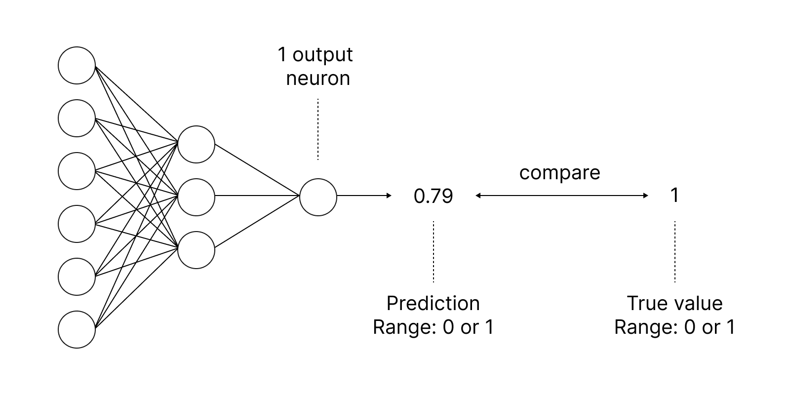
最流行的激活函数之一是 sigmoid。
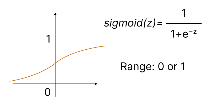
内置的 Activation 方法能够设置激活函数的十五种类型之一。 所有这些都在 ENUM_ACTIVATION_FUNCTION 枚举中列出。
| ID | 说明 |
|---|---|
| AF_ELU | 指数线性单元 |
| AF_EXP | 指数 |
| AF_GELU | 高斯误差线性单元 |
| AF_HARD_SIGMOID | 强硬 Sigmoid |
| AF_LINEAR | 线性 |
| AF_LRELU | 泄露修正线性单元( |
| AF_RELU | 修正线性单元( |
| AF_SELU | 缩放指数线性单位 |
| AF_SIGMOID | Sigmoid |
| AF_SOFTMAX | Softmax |
| AF_SOFTPLUS | Softplus |
| AF_SOFTSIGN | Softsign |
| AF_SWISH | Swish |
| AF_TANH | 双曲正切函数 |
| AF_TRELU | 阈值整流线性单元 |
神经网络旨在找到一种算法,从而令学习误差最小化,为此使用了损失函数。 偏差是调用 Loss 方法计算得出,您可以指定来自 ENUM_LOSS_FUNCTION 枚举中的 14 种类型之一。
生成的偏差值随后用来细化神经网络参数。 这是调用 Derivative 方法完成的,该方法计算激活函数的导数值,并将结果写入所传递的向量/矩阵。 神经网络训练过程可参见文章“使用 MQL 语言从头开始深度神经网络编程”中的动画直观地表示。
基于 OpenCL 的改进
我们还在 CLBufferWrite 和 CLBufferRead 函数中实现了矩阵和矢量的支持。 并已为这些函数提供了相应的重载。 矩阵的示例如下所示。
将来自矩阵的数值写入缓冲区,并在成功后返回 true。
uint  CLBufferWrite(
   int           buffer,                    // OpenCL buffer handle
   uint          buffer_offset,             // offset in the OpenCL buffer in bytes
   matrix<T>     &mat                       // matrix of values to write to buffer
   );
读取 OpenCL 缓冲区至矩阵,并在成功后返回 true。
uint  CLBufferRead(
   int           buffer,                    // OpenCL buffer handle
   uint          buffer_offset,             // offset in the OpenCL buffer in bytes
   const matrix& mat,                       // matrix to get values from the buffer
   ulong         rows=-1,                   // number of rows in the matrix
   ulong         cols=-1                    // number of columns in the matrix
   );
我们利用矩阵乘积示例来研究两个新重载函数的用法。 我们可用三种方法进行计算:
- 描绘矩阵乘法算法的一种稚嫩方法
- 内置 MatMul 方法
- OpenCL 中的并行计算
所获矩阵将调用 Compare 方法进行检查,该方法以给定的精度比较两个矩阵的元素。
#define M       3000      // number of rows in the first matrix
#define K       2000      // number of columns in the first matrix equal to the number of rows in the second one
#define N       3000      // number of columns in the second matrix

//+------------------------------------------------------------------+
const string clSrc=
  "#define N     "+IntegerToString(N)+"                              \r\n"
  "#define K     "+IntegerToString(K)+"                              \r\n"
  "                                                                  \r\n"
  "__kernel void matricesMul( __global float *in1,                   \r\n"
  "                           __global float *in2,                   \r\n"
  "                           __global float *out  )                 \r\n"
  "{                                                                 \r\n"
  "  int m = get_global_id( 0 );                                     \r\n"
  "  int n = get_global_id( 1 );                                     \r\n"
  "  float sum = 0.0;                                                \r\n"
  "  for( int k = 0; k < K; k ++ )                                   \r\n"
  "     sum += in1[ m * K + k ] * in2[ k * N + n ];                  \r\n"
  "  out[ m * N + n ] = sum;                                         \r\n"
  "}                                                                 \r\n";
//+------------------------------------------------------------------+
//| Script program start function                                    |
//+------------------------------------------------------------------+
void OnStart()
 {
//--- initialize the random number generator
  MathSrand((int)TimeCurrent());
//--- fill matrices of the given size with random values
  matrixf mat1(M, K, MatrixRandom) ;    // first matrix
  matrixf mat2(K, N, MatrixRandom);     // second matrix

//--- calculate the product of matrices using the naive way
  uint start=GetTickCount();
  matrixf matrix_naive=matrixf::Zeros(M, N);// here we rite the result of multiplying two matrices
  for(int m=0; m<M; m++)
    for(int k=0; k<K; k++)
      for(int n=0; n<N; n++)
        matrix_naive[m][n]+=mat1[m][k]*mat2[k][n];
  uint time_naive=GetTickCount()-start;

//--- calculate the product of matrices using MatMull
  start=GetTickCount();
  matrixf matrix_matmul=mat1.MatMul(mat2);
  uint time_matmul=GetTickCount()-start;

//--- calculate the product of matrices in OpenCL
  matrixf matrix_opencl=matrixf::Zeros(M, N);
  int cl_ctx;             // context handle
  if((cl_ctx=CLContextCreate(CL_USE_GPU_ONLY))==INVALID_HANDLE)
   {
    Print("OpenCL not found, exit");
    return;
   }
  int cl_prg;             // program handle
  int cl_krn;             // kernel handle
  int cl_mem_in1;         // handle of the first buffer (input)
  int cl_mem_in2;         // handle of the second buffer (input)
  int cl_mem_out;         // handle of the third buffer (output)
//--- create the program and the kernel
  cl_prg = CLProgramCreate(cl_ctx, clSrc);
  cl_krn = CLKernelCreate(cl_prg, "matricesMul");
//--- create all three buffers for the three matrices
  cl_mem_in1=CLBufferCreate(cl_ctx, M*K*sizeof(float), CL_MEM_READ_WRITE);
  cl_mem_in2=CLBufferCreate(cl_ctx, K*N*sizeof(float), CL_MEM_READ_WRITE);
//--- third matrix - output
  cl_mem_out=CLBufferCreate(cl_ctx, M*N*sizeof(float), CL_MEM_READ_WRITE);
//--- set kernel arguments
  CLSetKernelArgMem(cl_krn, 0, cl_mem_in1);
  CLSetKernelArgMem(cl_krn, 1, cl_mem_in2);
  CLSetKernelArgMem(cl_krn, 2, cl_mem_out);
//--- write matrices to device buffers
  CLBufferWrite(cl_mem_in1, 0, mat1);
  CLBufferWrite(cl_mem_in2, 0, mat2);
  CLBufferWrite(cl_mem_out, 0, matrix_opencl);
//--- start the OpenCL code execution time
  start=GetTickCount();
//--- set the task workspace parameters and execute the OpenCL program
  uint  offs[2] = {0, 0};
  uint works[2] = {M, N};
  start=GetTickCount();
  bool ex=CLExecute(cl_krn, 2, offs, works);
//--- read the result into the matrix
  if(CLBufferRead(cl_mem_out, 0, matrix_opencl))
    PrintFormat("Matrix [%d x %d] read ", matrix_opencl.Rows(), matrix_opencl.Cols());
   else
      Print("CLBufferRead(cl_mem_out, 0, matrix_opencl failed. Error ",GetLastError());
  uint time_opencl=GetTickCount()-start;
  Print("Compare computation times of the methods");
  PrintFormat("Naive product time = %d ms",time_naive);
  PrintFormat("MatMul product time = %d ms",time_matmul);
  PrintFormat("OpenCl product time = %d ms",time_opencl);
//--- release all OpenCL contexts
  CLFreeAll(cl_ctx, cl_prg, cl_krn, cl_mem_in1, cl_mem_in2, cl_mem_out);

//--- compare all obtained result matrices with each other
  Print("How many discrepancy errors between result matrices?");
  ulong errors=matrix_naive.Compare(matrix_matmul,(float)1e-12);
  Print("matrix_direct.Compare(matrix_matmul,1e-12)=",errors);
  errors=matrix_matmul.Compare(matrix_opencl,float(1e-12));
  Print("matrix_matmul.Compare(matrix_opencl,1e-12)=",errors);
/*
   Result:

   Matrix [3000 x 3000] read
   Compare computation times of the methods
   Naive product time = 54750 ms
   MatMul product time = 4578 ms
   OpenCl product time = 922 ms
   How many discrepancy errors between result matrices?
   matrix_direct.Compare(matrix_matmul,1e-12)=0
   matrix_matmul.Compare(matrix_opencl,1e-12)=0
*/
 }
//+------------------------------------------------------------------+
//| Fills the matrix with random values                              |
//+------------------------------------------------------------------+
void MatrixRandom(matrixf& m)
 {
  for(ulong r=0; r<m.Rows(); r++)
   {
    for(ulong c=0; c<m.Cols(); c++)
     {
      m[r][c]=(float)((MathRand()-16383.5)/32767.);
     }
   }
 }
//+------------------------------------------------------------------+
//| Release all OpenCL contexts                                      |
//+------------------------------------------------------------------+
void CLFreeAll(int cl_ctx, int cl_prg, int cl_krn,
               int cl_mem_in1, int cl_mem_in2, int cl_mem_out)
 {
//--- release all created OpenCL contexts in reverse order
  CLBufferFree(cl_mem_in1);
  CLBufferFree(cl_mem_in2);
  CLBufferFree(cl_mem_out);
  CLKernelFree(cl_krn);
  CLProgramFree(cl_prg);
  CLContextFree(cl_ctx);
 }
来自 “OpenCL:从稚嫩到更有见地的编码” 文章中示例提供的 OpenCL 代码详解。
更多改进
Build 3390 解除了 OpenCL 操作中的两个限制,原来的这些限制影响了 GPU 的使用。
为了针对特定任务,强制设置 GPU 采用精度支持,请以 CL_USE_GPU_DOUBLE_ONLY 为参数调用 CLContextCreate。
   int cl_ctx;
//--- initialization of OpenCL context
   if((cl_ctx=CLContextCreate(CL_USE_GPU_DOUBLE_ONLY))==INVALID_HANDLE)
     {
      Print("OpenCL not found");
      return;
     }
尽管 OpenCL 操作的变化与矩阵和向量没有直接关系,但它们与我们开发 MQL5 语言机器学习功能的努力是一致的。
MQL5 在机器学习中的未来
在过去的几年里,我们已在 MQL5 语言里引入先进技术方面做了很多工作:
- 将 ALGLIB 数值方法库植入 MQL5
- 实现了一个运用模糊逻辑和统计方法的数学库
- 引入图形库,类似于绘图功能
- 集成 Python,并可直接在终端中运行 Python 脚本
- 添加 DirectX 函数来创建 3D 图形
- 实现原生 SQLite 支持,从而支持数据库的操作
- 添加新的数据类型:=矩阵和向量,以及所有必要的方法
MQL5 语言还将继续发展,而机器学习是重中之重。 我们已制定了进一步发展的大计划。 故此,继续关注我们,支持我们,我们一起不断进取。