
Cluster analysis (Part I): Mastering the slope of indicator lines

Abstract
Cluster analysis is one of the most important elements of artificial intelligence. What is observed, usually in the form of tuples of numbers or points, is grouped into clusters or heaps. The goal is, by successfully assigning an observed point to a cluster or category, to assign the known properties of that category to the observed new point, and then act accordingly. The goal here will be to see if and how well the slope of an indicator tells us if the market is flat, or following a trend.
Numbering and naming convention
The indicator "HalfTrend" that is used as an example is built in the tradition of MQL4 so that the index of bars or candles (iB) on the price chart counts from its largest value (rates_total), the index of the oldest bar down to zero, the newest and the current bar. The first time the OnCalculate() function is called after the indicator is started, the value of prev_calculated is zero, since nothing has been calculated yet; on subsequent calls, it can be used to detect which bars have already been calculated and which have not.
The indicator uses a two-color indicator line, which is realized by two data buffers up[] and down[] - each with its own color. Only one of the two buffers receives a valid value greater than zero at a time, the other is assigned zero at the same position (buffer element with the same index iB), and this means it is not drawn.
In order to make the further use of this cluster analysis for other indicators or programs as simple as possible, as few additions as possible were made to the HalfTrend indicator. The added lines are 'bracketed' in the code of the indicator by the following comments:
//+------------------------------------------------------------------+
//| added for cluster analysis                                       |
//+------------------------------------------------------------------+
....
//+------------------------------------------------------------------+
The functions and data of the cluster analysis you find completely in the file ClusterTrend.mqh, which is attached below. The basis of the whole calculation is the following data structure of all clusters:
struct __IncrStdDev
  {
   double µ,       // average
          σ,       // standard deviation
          max,min, // max. and min. values
          S2;      // auxiliary variable
   uint   ID,n;    // ID and no. of values
  };
µ is the mean, σ is the standard deviation - the root of the variance, it indicates how close the values in the cluster vary around the mean -- max and min are respectively the largest and smallest values in the cluster and S2 is an auxiliary variable. n is the number of values in the cluster and ID is the identifier of the cluster.
This data structure is organized in a two-dimensional array:
__cluster cluster[][14];
Since in MQL5 only the first dimension of multidimensional arrays can be dynamically adjusted, the number of value types to be examined is assigned to it. So it can be easily changed. The second dimension is the number of classification values, which are fixed in the following one-dimensional array:
double CatCoeff[9] = {0.0,0.33,0.76,1.32,2.04,2.98,4.21,5.80,7.87};
Both lines are immediately below each other because the number of coefficients in CatCoeff conditions the fixed size of the second dimension of Cluster, it must be greater by 5. The reason will be explained below. Since both arrays condition each other, they can easily be changed together.
Only the difference of an indicator value and its previous value is examined: x[iB] - x[iB+1]. These differences are converted into points (_Point), in order to enable the comparability of different trading instruments such as EURUSD with 5 decimal places and XAUUSD (gold) with only two decimal places.
The challenge
To trade, it is essential to know whether the market is flat or has a weak or strong trend. In a sideways movement, one would trade from the boundary of a channel around a suitable average indicator back to the indicator, back to the centre of the channel, whereas in a trend, one must trade in the direction of the trend away from the average indicator, away from the centre of the channel, i.e. exactly the other way around. A near-perfect indicator used by an EA would therefore need to clearly separate these two states. An EA needs a number in which the market action is reflected, and it needs thresholds to know in this case whether the number of the indicator signals a trend or a flat. Visually, it often seems easy to make an assessment in this regard. But the visual feeling is often difficult to concretize into a formula and/or a number. The cluster analysis is a mathematical method of grouping data or assigning them to categories. It will help us to separate these two states of the market.Cluster analysis defines or achieves through optimization:
- the number of clusters
- the centers of the clusters
- the allocation of the points to only one of the clusters - if possible (= no overlapping clusters).
- that all or as many as possible (maybe except for outliers) of the number tuples can be assigned to one cluster,
- that the size of the clusters is as small as possible
- that they overlap as little as possible (then it would not be clear whether a point would belong to one or its neighboring cluster),
- that the number of clusters is as small as possible.
This leads to the fact that especially with many points, values or elements and many clusters the matter can become computationally very expensive.
The O-notation
The representation of the computational effort is in the form of the O-notation. O(n) means for example that here the computation needs to access all n elements only once. Well-known examples of the importance of this quantity are the values for sorting algorithms. The fastest ones normally have an O(nlog(n)), the slowest ones O(n²). Not only in former times this was an important criterion for large amounts of data and for computers which were not so fast at that time. Today, computers are many times faster, but at the same time, in some areas, the amount of data (the optical analysis of the environment and the object categorization) has increased too very much.
The first and most famous algorithm in cluster analysis is k-means. It assigns n observations or vectors with d dimensions to k clusters by minimizing the (Euclidean) distances to the centers of the clusters. This leads to computational cost of O(n^(dk+1)). We have only one dimension d, the respective indicator difference to the previous value, but the whole price history of e.g. a demo account of MQ for GBPUSD D1 (daily) candles includes 7265 bars or candles of quotes, the n in the formula. Since we do not know at the beginning how many clusters are useful or we need, I use k=9 clusters or categories. According to this relation, this would lead to an effort of O(7265^(1*9+1)) or O(4,1*10^38). Much too much for normal trading computers. With the way presented here it is possible to achieve the clustering in 16 mSec, which would be 454.063 values per second. When calculating bars of GBPUSD m15 (bars of 15 minutes) with this program we have 556.388 bars and again 9 cluster and it takes 140 mSec or 3.974.200 values per second. It shows that clustering is even better than O(n) which can be justified by the way the terminal of MQ organizes the data, because after all the computational effort to calculate the indicator also flows into this period.
The Indicator
As an indicator I use "HalfTrend" from MQ, which is attached below. It has longer passages in which it runs horizontally:

My question to this indicator now was whether there is a clear separation, i.e. threshold, which can be interpreted as a sign for flat and a threshold signaling a trend, be it up or down. Of course, everyone immediately sees that if this indicator is exactly horizontal, the market is flat. But up to which height of the slope are the changes in the market so small that the market is still to be considered flat and from which height one must assume a trend. Imagine the EA sees only one number, in which the whole chart picture is concentrated and not, as we see in the picture above, the bigger picture. This will be solved by the cluster analysis. But before we turn to the cluster analysis, we first consider the changes that were made in the Indicator.
Changes in the Indicator
Since the indicator should be changed as little as possible, the clustering has been moved to an external file ClusterTrend.mqh, which is included at the beginning of the indicator with;
Of course this file is attached. But this alone is not enough. To make your own attempts as easy as possible, the input variable NumValues was added:
input int NumValues = 1;
This value 1 means that (only) one value type should be examined. For example, if you want to analyze an indicator that calculates two averages and you want to evaluate the slope of both and thirdly the distance between these two NumValues should be set to 3. The array over which the calculation is made is then automatically adjusted. If the value is set to zero, no cluster analysis is performed. So this additional load can easily be turned off by the settings.
Furthermore there are the global variables
string ShortName;
long StopWatch=0;
ShortName is assigned the short name of the indicator in OnInit():
ShortName = "HalfTrd "+(string)Amplitude;
IndicatorSetString(INDICATOR_SHORTNAME,ShortName);
which will be used for identification when printing the results.
StopWatch is used for timing and is set immediately before the first value is passed for cluster analysis and is read after the results are printed:
if (StopWatch==0) StopWatch = GetTickCount64();
...
if (StopWatch!=0) StopWatch = GetTickCount64()-StopWatch;
Like almost all indicators, this one has a big loop over all available bars of the price history. This indicator calculates its values so that the bar on the chart with index iB=0, contains the current, most recently received prices, while the largest possible index represents the beginning of the price history, the oldest bars. As the last thing before the end of this loop, the closing bracket, the value to be analysed is calculated and passed to the cluster function for evaluation. There everything is automated. It will be explained further below.
In the code block right before the end of the loop, the first thing that is done is to make sure that the cluster analysis with the historical prices is done only once for each bar and not every time a new price arrives:
//+------------------------------------------------------------------+
//| added for cluster analysis |
//+------------------------------------------------------------------+
if ( (prev_calculated == 0 && iB > 0 ) // we don't use the actual bar
|| (prev_calculated > 9 && iB == 1)) // during operation we use the second to last bar: iB = 1
{
Then we check that its the very first bar of the initialization to set the stopwatch and to nullify prev. results (if any):
if (prev_calculated==0 && iB==limit) { // only at the very first pass/bar
StopWatch = GetTickCount64(); // start the stop whatch
if (ArraySize(Cluster) > 0) ArrayResize(Cluster,0); // in case everything is recalculated delete prev. results
}
Then the indicator value is determined with the bar index iB and that of the previous bar (iB+1). Since this indicator line is two-colored (see above) and this was realized with the two buffers up[] and down[], where one is always 0,0 and therefore not drawn, the indicator value, is the one of the two buffers that is greater than zero:
double actBar = fmax(up[iB], down[iB]), // get actual indi. value of bar[iB]
prvBar = fmax(up[iB+1], down[iB+1]); // get prev. indi. value
To make sure that the cluster analysis is affected with values at the beginning of the calculation, although the indicator has not been calculated at all, there is this safety check:
if ( (actBar+prvBar) < _Point ) continue; // skip initially or intermediately missing quotes
Now we can pass the absolute difference from the indicator value and its previous value.
enterVal(fabs(actBar-prvBar)/_Point, // abs. of slope of the indi. line
0, // index of the value type
1.0 - (double)iB/(double)rates_total, // learning rate: use either 1-iB/rates_total or iB/rates_total whatever runs from 0 .. 1
NumValues // used for initialization (no. of value types) and if < 1 no clustering
);
Why do we use in the first argument the absolute difference fabs(actBar-prvBar)? If we passed the pure difference, we would have to determine twice the number of clusters, those for greater than zero and those for less than zero. Then it would also become relevant whether a price has risen or fallen overall within the available price history, and that could skew the results. Ultimately, what matters (to me) is the strength of a slope, not its direction. In the forex market, I think it is reasonable to assume that the ups and downs of prices are somewhat equivalent - perhaps different than in the stock market.
The second argument, 0, is the index of the type of value passed (0=the first, 1=the second,..). With i.e. two indicator lines and their difference, we would need to set 0, 1, and 2 for the respective value.
The third argument
1.0 - (double)iB/(double)rates_total, // learning rate: use either 1-iB/rates_total or iB/rates_total whatever runs from 0 .. 1
concerns the learning rate. The index iB runs from the largest value down to 0. rates_total is the total number of all bars. Thus, iB/rates_total is the ratio of what has not yet been computed and falls from almost 1 (nothing computed) to zero (everything computed) and therefore 1 minus this value increases from almost 0 (nothing learned yet) to 1 (done). The importance of this ratio is explained below.
The last parameter is needed for initialization and whether the clusters should be calculated. If it is greater than zero, it specifies (see above) the number of value types, e.g. indicator lines, and thus determines the size of the first dimension of the global array Cluster[]][] in the file ClusterTrend.mqh (see above).
Right after the end of the large loop over the entire price history, all the results are printed to the expert tab by one line for each category/cluster:
prtStdDev(_Symbol+" "+EnumToString(Period())+" "+ShortName, // printed at the beginning of each line
0, // the value type to be printed
NumValues); // if <=0 this value type is not printed
Here the first argument is for information and is printed at the beginning of each line, the second, 0, denotes the calculated indicator type (0=the first, 1=the second,..) and finally as above NumValues. If it is 0, this indicator type is not printed.
Overall, the added block looks like this:
      //+------------------------------------------------------------------+
      //|  added for cluster analysis                                      |
      //+------------------------------------------------------------------+
      if (  (prev_calculated == 0 && iB > 0 )                        // we don't use the actual bar
         || (prev_calculated > 9 && iB == 1))                        // during operation we use the second to last bar: iB = 1

       {
         if (prev_calculated==0 && iB==limit) {                      // only at the very first pass/bar
            StopWatch = GetTickCount64();                            // start the stop whatch
            if (ArraySize(Cluster) > 0) ArrayResize(Cluster,0);      // in case everything is recalculated delete prev. results
         }
         double actBar = fmax(up[iB], down[iB]),                     // get actual indi. value of bar[iB]
                prvBar = fmax(up[iB+1], down[iB+1]);                 // get prev. indi. value
         if ( (actBar+prvBar) < _Point ) continue;                   // skip initially or intermediately missing quotes
         enterVal(fabs(actBar-prvBar)/_Point,                        // abs. of slope of the indi. line
                  0,                                                 // index of the value type
                  1.0 - (double)iB/(double)rates_total,              // learning rate: use either 1-iB/rates_total or iB/rates_total whatever runs from 0 .. 1
                  NumValues                                          // used for initialization (no. of value types) and if < 1 no clustering
         );
       }
      //+------------------------------------------------------------------+

   } // end of big loop: for(iB = limit; iB >= 0; iB--) ..

   //+------------------------------------------------------------------+
   //|  added for cluster analysis                                      |
   //+------------------------------------------------------------------+
   if (prev_calculated < 1)                                          // print only once after initialization
    {
      prtStdDev(_Symbol+" "+EnumToString(Period())+" "+ShortName,    // printed at the beginning of each line
                0,                                                   // the value type to be printed
                NumValues);                                          // if <=0 this value type is not printed
      if (StopWatch!=0) StopWatch = GetTickCount64()-StopWatch;
      Print ("Time needed for ",rates_total," bars on a PC with ",TerminalInfoInteger(TERMINAL_CPU_CORES),
             " cores and Ram: ",TerminalInfoInteger(TERMINAL_MEMORY_PHYSICAL),", Time: ",
             TimeToString(StopWatch/1000,TIME_SECONDS),":",StringFormat("%03i",StopWatch%1000) );
    }
   //+------------------------------------------------------------------+
These are all the changes in the indicator.
The cluster analysis in the ClusterTrend.mqh file
The file is located in the same folder as the indicator, so it must be included in the form "ClusterTrend.mqh".
At the beginning there are some simplifications with #define. #define crash(strng) artificially provokes a division by 0, which the compiler does not recognize, as it is actually (still?) impossible for an indicator program to terminate itself. This does not quite succeed with this either, but at least the alert() claiming wrong dimension specification is called only once. Correct it and recompile you indicator.
The structure of the data used for this analysis has already been described above.
Now let's get to the core of the idea of this approach.
Actually, mean, variance, and also the cluster analysis are calculated with data that must be available in total. Firstly, the data must be collected, and then in a second step these values and the clustering are done by one or more loops. Traditionally, the average of all previous values arriving one by one would be calculated with a second loop in the big one overall data to sum up. This would be very time consuming. But I have found a publication by Tony Finch: "Incremental calculation of weighted mean and variance", in which he calculates mean and variance incrementally, that is, in one pass through all the data, instead of summing up all data and then dividing the sum by the number of values. The new (simple) mean over all previous values including the newly transmitted one is thus calculated according to the formula (4), p.1:
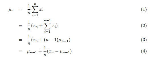
where:
- µn = the updated mean value,
- µn-1 = the previous mean value,
- n = the current number (including the new one) of values,
- xn = the new, nth value.
Even the variance is calculated on-the-fly instead of in a second loop after the mean. The incremental variance is then calculated (formula 24,25; p. 3):
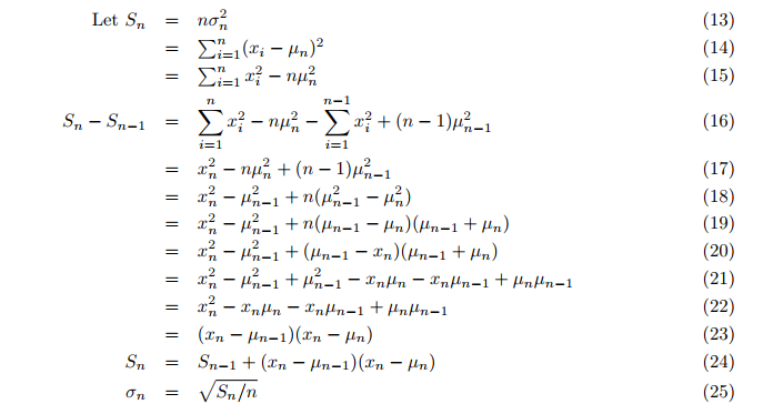
Where:
- Sn = updated value of the auxiliary variable S,
- σ = the variance.
Thus, the mean and variance of the population can be calculated in one pass, each time up-to-date for the most recent, new value in the function incrStdDeviation(..):
On this basis, an average value calculated in this way can already be used for classification after a first part of the historical data. You may ask, why can't we use simply a moving average, which achieves useful results with little amount of data, quick and easy? A moving average adjusts. But for the goal of a classification we need a relatively constant comparison value. Just imagine that the water level of a river is to be measured. It is clear that the comparison value of the normal water level must not change with the current height. In times with strong trends, for example, the differences of the moving average would also increase and the differences to this value would become unjustifiably smaller. And when the market becomes flat, the average also decreases and this would realtively increase the difference to this base value. So we need a very stable value, just an average of as much as possible.
Now the question of clustering arises. Traditionally, one would again use all values to form clusters. Well, the incremental calculation of the mean value gives us another possibility: We use the oldest 50% of the historical data for the mean value and the newest 50% for the clustering (continuing the calculation of the mean value). This percentage (50%) is here called the learning rate, in the sense that up to 50% only the mean value is 'learned'. However, its calculation is not stopped after reaching the 50%, but it is now so stable that it produces good results. Nevertheless, the number 50% remains my arbitrary decision, so I have made two other mean values for comparison: 25% and 75%.They start calculating their mean value after their learning rate has been reached. With this, we can see how and how much the slope has changed.
Creating mean and cluster
Almost everthing is managed by the function enterVal() of the file ClusterTrend.mqh:
//+------------------------------------------------------------------+
//|                                                                  |
//| enter a new value                                                |
//|                                                                  |
//+------------------------------------------------------------------+
// use; enterVal( fabs(indi[i]-indi[i-1]), 0, (double)iB/(double)rates_total )
void enterVal(const double val, const int iLne, const double learn, const int NoVal)
  {
   if (NoVal<=0) return;                              // nothing to do if true
   if(   ArrayRange(Cluster,0)<NoVal
      || Cluster[iLne][0].n <= 0 )                    // need to inicialize
      setStattID(NoVal);


   incrStdDeviation(val, Cluster[iLne][0]);           // the calculation from the first to the last bar

   if(learn>0.25)
      incrStdDeviation(val, Cluster[iLne][1]);        // how does µ varies after 25% of all bars
   if(learn>0.5)
      incrStdDeviation(val, Cluster[iLne][2]);        // how does µ varies after 50% of all bars
   if(learn>0.75)
      incrStdDeviation(val, Cluster[iLne][3]);        // how does µ varies after 75% of all bars


   if(learn<0.5)
      return;                                         // I use 50% to learn and 50% to devellop the categories
   int i;
   if (Cluster[iLne][0].µ < _Point) return;           // avoid division by zero
   double pc = val/(Cluster[iLne][0].µ);              // '%'-value of the new value compared to the long term µ of Cluster[0]..
   for(i=0; i<ArraySize(CatCoeff); i++)
     {
      if(pc <= CatCoeff[i])
        {
         incrStdDeviation(val, Cluster[iLne][i+4]);   // find the right category
         return;
        }
     }
   i = ArraySize(CatCoeff);
   incrStdDeviation(val, Cluster[iLne][i+4]);         // tooo big? it goes to the last category
  }
val is the value received from the indicator, iLine is the index of the value type, learn is the learning rate or the ratio of done/history and finally NoVal allows us to know how many - if any - value types are to be calculated.
At first is a test (NoVal<=0) whether a clustering is intended or not.
Followed by the check (ArrayRange(Cluster,0) < NoVal) whether the first dimension of the array Cluster[][] has the size of the value types to be calculated. If not, the initialization is performed, all values are set to zero, and the ID is assigned by the function setStattID(NoVal) (see below).
I want to keep the amount of code low in order to make it easy for others to use it and for me to understand it again after some time I have not worked with it. Therefore, the value val is assigned to the corresponding data structure via one and the same function incrStdDeviation(val, Cluster[][]) and processed there.
The incrStdDeviation(val, Cluster[iLne][0]) function calculates the mean from the first to the last value. As already mentioned, the first index [iLine] denotes the value type and the second index [0] denotes the data structure of the value type for the calculation. As known from above, we need 5 more than the amount of elements in the static array CatCoeff[9]. Now we see why:
- [0] .. [3] are needed for the different means [0]:100%, [1]:25%, [2]:50%, [3]:75%,
- [4] .. [12] are needed for the 9 categories of CatCoeff[9]: 0.0, .., 7.87
- [13] is needed as the last category for values that are larger than the largest category of CatCoeff[8] (here 7.87).
Now we can understand for what we need a stable mean value. To find the category or cluster we calculate the ration of val/Cluster[iLne][0].µ. This is the overall mean of the value type with the index iLine. Therefore the coefficients of the array CatCoeff[] are thus multipliers of the overall mean value if we transform the equation:
pc = val/µ => pc*µ = val
This means systematically that we have not only predefined the number of clusters (most clustering methods require this), we have also predefined the properties of the clusters and this is rather unusual, but this is the reason why this clustering method needs only one pass, while the other methods need several passes over all data to find the optimal properties of the clusters (see above).The very first coefficient of (CatCoeff[0]) is zero. This is chosen because the indicator "HalfTrend" is designed to run horizontally for multiple bars and so the difference of the indicator values are then zero. So it is expected that this category will reach a significant size. All other assignments are made if:
pc <= CatCoeff[i] => val/µ <= CatCoeff[i] => val <= CatCoeff[i]*µ.
Since there are certainly outliers that would blow up the given categories in CatCoeff[], there is an additional category for such values:
i = ArraySize(CatCoeff);
incrStdDeviation(val, Cluster[iLne][i+4]); // tooo big? it goes to the last category
Evaluation and printout
Right after the end of the big loop of the idicator and only if it is the first pass (prev_calculated < 1), the results are printed into the journal by prtStdDev(), then the StopWatch is stopped, and printed as well (s.a):
   //+------------------------------------------------------------------+
   //|  added for cluster analysis                                      |
   //+------------------------------------------------------------------+
   if (prev_calculated < 1)
    {
      prtStdDev(_Symbol+" "+EnumToString(Period())+" "+ShortName, 0, NumValues);
      if (StopWatch!=0) StopWatch = GetTickCount64()-StopWatch;
      Print ("Time needed for ",rates_total," bars on a PC with ",TerminalInfoInteger(TERMINAL_CPU_CORES),
             " cores and ",TerminalInfoInteger(TERMINAL_MEMORY_PHYSICAL)," Ram: ",TimeToString(StopWatch/1000,TIME_SECONDS));
    }
   //+------------------------------------------------------------------+
prtStdDev(..) prints at first the headline with HeadLineIncrStat(pre) and then for each value type (index iLine) all 14 results in one line each using retIncrStat():
void prtStdDev(const string pre, int iLne, const int NoVal)
  {
   if (NoVal <= 0 ) return;                               // if true no printing
   if (Cluster[iLne][0].n==0 ) return;                    // no values entered for this 'line'
   HeadLineIncrStat(pre);                                 // print the headline
   int i,tot = 0,sA=ArrayRange(Cluster,1),
       sC=ArraySize(CatCoeff);
   for(i=4; i<sA; i++)
      tot += (int)Cluster[iLne][i].n;                     //  sum up the total volume of all but the first [0] category

   retIncrStat(Cluster[iLne][0].n, pre, "learn 100% all["+(string)sC+"]", Cluster[iLne][0], 1, Cluster[iLne][0].µ); // print the base the first category [0]
   retIncrStat(Cluster[iLne][1].n, pre, "learn  25% all["+(string)sC+"]", Cluster[iLne][1], 1, Cluster[iLne][0].µ); // print the base the first category [0]
   retIncrStat(Cluster[iLne][2].n, pre, "learn  50% all["+(string)sC+"]", Cluster[iLne][2], 1, Cluster[iLne][0].µ); // print the base the first category [0]
   retIncrStat(Cluster[iLne][3].n, pre, "learn  75% all["+(string)sC+"]", Cluster[iLne][3], 1, Cluster[iLne][0].µ); // print the base the first category [0]

   for(i=4; i<sA-1; i++)
     {
      retIncrStat(tot, pre,"Cluster["+(string)(i)+"] (<="+_d22(CatCoeff[i-4])+")", Cluster[iLne][i], 1, Cluster[iLne][0].µ);           // print each category
     }
   retIncrStat(tot, pre,"Cluster["+(string)i+"] (> "+_d22(CatCoeff[sC-1])+")", Cluster[iLne][i], 1, Cluster[iLne][0].µ);         // print the last category
  }
Here: tot += (int)Cluster[iLne][i].n is the number of values in the categories 4-13 summed up in order to have a comparison value (100%) for these categories. And this is what we get by the printout:
GBPUSD PERIOD_D1 HalfTrd 2          ID                Cluster      Num. (tot  %)          µ   (mult*µ)            σ (Range %)           min -          max
GBPUSD PERIOD_D1 HalfTrd 2      100100      learn 100% all[9]      7266 (100.0%)      217.6   (1.00*µ)       1800.0   (1.21%)           0.0 -     148850.0
GBPUSD PERIOD_D1 HalfTrd 2      100025      learn  25% all[9]      5476 (100.0%)      212.8   (0.98*µ)        470.2   (4.06%)           0.0 -      11574.0
GBPUSD PERIOD_D1 HalfTrd 2      100050      learn  50% all[9]      3650 (100.0%)      213.4   (0.98*µ)        489.2   (4.23%)           0.0 -      11574.0
GBPUSD PERIOD_D1 HalfTrd 2      100075      learn  75% all[9]      1825 (100.0%)      182.0   (0.84*µ)        451.4   (3.90%)           0.0 -      11574.0
GBPUSD PERIOD_D1 HalfTrd 2      400000    Cluster[4] (<=0.00)      2410 ( 66.0%)        0.0   (0.00*µ)          0.0                     0.0 -          0.0
GBPUSD PERIOD_D1 HalfTrd 2      500033    Cluster[5] (<=0.33)       112 (  3.1%)       37.9   (0.17*µ)         20.7  (27.66%)           1.0 -         76.0
GBPUSD PERIOD_D1 HalfTrd 2      600076    Cluster[6] (<=0.76)       146 (  4.0%)      124.9   (0.57*µ)         28.5  (26.40%)          75.0 -        183.0
GBPUSD PERIOD_D1 HalfTrd 2      700132    Cluster[7] (<=1.32)       171 (  4.7%)      233.3   (1.07*µ)         38.4  (28.06%)         167.0 -        304.0
GBPUSD PERIOD_D1 HalfTrd 2      800204    Cluster[8] (<=2.04)       192 (  5.3%)      378.4   (1.74*µ)         47.9  (25.23%)         292.0 -        482.0
GBPUSD PERIOD_D1 HalfTrd 2      900298    Cluster[9] (<=2.98)       189 (  5.2%)      566.3   (2.60*µ)         67.9  (26.73%)         456.0 -        710.0
GBPUSD PERIOD_D1 HalfTrd 2     1000421   Cluster[10] (<=4.21)       196 (  5.4%)      816.6   (3.75*µ)         78.9  (23.90%)         666.0 -        996.0
GBPUSD PERIOD_D1 HalfTrd 2     1100580   Cluster[11] (<=5.80)       114 (  3.1%)     1134.9   (5.22*µ)        100.2  (24.38%)         940.0 -       1351.0
GBPUSD PERIOD_D1 HalfTrd 2     1200787   Cluster[12] (<=7.87)        67 (  1.8%)     1512.1   (6.95*µ)        136.8  (26.56%)        1330.0 -       1845.0
GBPUSD PERIOD_D1 HalfTrd 2     1300999   Cluster[13] (> 7.87)        54 (  1.5%)     2707.3  (12.44*µ)       1414.0  (14.47%)        1803.0 -      11574.0
Time needed for 7302 bars on a PC with 12 cores and Ram: 65482, Time: 00:00:00:016
So what do we see? Let's go from column to column. The first column tells you the symbol, timeframe, the name of the indicator and its "Amplitude" as it was assigned to ShortName. The second column shows the ID of each data structure. The 100nnn shows it is just a mean calculation with the last three digits indicating the learning rate from, 100, 25, 50, and 75. 400nnn .. 1300nnn are the categories, clusters or heaps. Here the last three digits indicate the category or the multiplier for its mean µ which is shown as well in the third column under Cluster in parentheses. It is clear and self-explanatory.
Now it gets interesting. Column 4 shows the number of values in the respective category and the percentage in parentheses. The interesting thing here is that the indicator is horizontal most of the time (Cat.#4 2409 bars or days 66.0%), which suggests that one could succeed with range trading two-thirds of the time. But there are more (local) maxima in categories #8, #9 and #10, while category #5 received surprisingly few values (112, 3.1%). And this can now be interpreted as a gap between two thresholds and can provide us with the following rough values:
if fabs(slope) < 0.5*µ => the market is flat, try a range trading
if fabs(slope) > 1.0*µ => the market has a trend, try to ride the wave
The first 4 lines with IDs 100nnn help us estimate how stable µ is. As described, we do not need a value that fluctuates too much. We see that µ drops from 217.6 (points per day) at 100100 to 182.1 for 100075 (only the last 25% of the values are used for this µ) or 16%. A bit but not too much, I think. But what does this tell us? The volatility of GBPUSD has decreased. The first value in this category is dated 2014.05.28 00:00:00. Possibly this should be taken into account.
When a mean value is calculated, the variance σ shows valuable information and this brings us to column 6 (σ (Range %)). It indicates how close the individual values are to the mean value. For normally distributed values, 68% of all values lie within the variance. For the variance, this means the smaller the better or, in other words, the more accurate (less fuzzy) the mean value. Behind the value in parentheses is the ratio σ/(max-min) from the last two columns. This is also a measure of the quality of the variance and the mean.
Now let's see if the findings of GBPUSD D1 are repeated on smaller timeframes like M15 candles. For this, one has to simply switch the timeframe of the chart from D1 to M15:
GBPUSD PERIOD_M15 HalfTrd 2         ID                Cluster      Num. (tot  %)          µ   (mult*µ)            σ (Range %)           min -          max
GBPUSD PERIOD_M15 HalfTrd 2     100100      learn 100% all[9]    556389 (100.0%)       18.0   (1.00*µ)        212.0   (0.14%)           0.0 -     152900.0
GBPUSD PERIOD_M15 HalfTrd 2     100025      learn  25% all[9]    417293 (100.0%)       18.2   (1.01*µ)         52.2   (1.76%)           0.0 -       2971.0
GBPUSD PERIOD_M15 HalfTrd 2     100050      learn  50% all[9]    278195 (100.0%)       15.9   (0.88*µ)         45.0   (1.51%)           0.0 -       2971.0
GBPUSD PERIOD_M15 HalfTrd 2     100075      learn  75% all[9]    139097 (100.0%)       15.7   (0.87*µ)         46.1   (1.55%)           0.0 -       2971.0
GBPUSD PERIOD_M15 HalfTrd 2     400000    Cluster[4] (<=0.00)    193164 ( 69.4%)        0.0   (0.00*µ)          0.0                     0.0 -          0.0
GBPUSD PERIOD_M15 HalfTrd 2     500033    Cluster[5] (<=0.33)     10528 (  3.8%)        3.3   (0.18*µ)          1.7  (33.57%)           1.0 -          6.0
GBPUSD PERIOD_M15 HalfTrd 2     600076    Cluster[6] (<=0.76)     12797 (  4.6%)       10.3   (0.57*µ)          2.4  (26.24%)           6.0 -         15.0
GBPUSD PERIOD_M15 HalfTrd 2     700132    Cluster[7] (<=1.32)     12981 (  4.7%)       19.6   (1.09*µ)          3.1  (25.90%)          14.0 -         26.0
GBPUSD PERIOD_M15 HalfTrd 2     800204    Cluster[8] (<=2.04)     12527 (  4.5%)       31.6   (1.75*µ)          4.2  (24.69%)          24.0 -         41.0
GBPUSD PERIOD_M15 HalfTrd 2     900298    Cluster[9] (<=2.98)     11067 (  4.0%)       47.3   (2.62*µ)          5.5  (23.91%)          37.0 -         60.0
GBPUSD PERIOD_M15 HalfTrd 2    1000421   Cluster[10] (<=4.21)      8931 (  3.2%)       67.6   (3.75*µ)          7.3  (23.59%)          54.0 -         85.0
GBPUSD PERIOD_M15 HalfTrd 2    1100580   Cluster[11] (<=5.80)      6464 (  2.3%)       94.4   (5.23*µ)          9.7  (23.65%)          77.0 -        118.0
GBPUSD PERIOD_M15 HalfTrd 2    1200787   Cluster[12] (<=7.87)      4390 (  1.6%)      128.4   (7.12*µ)         12.6  (22.94%)         105.0 -        160.0
GBPUSD PERIOD_M15 HalfTrd 2    1300999   Cluster[13] (> 7.87)      5346 (  1.9%)      241.8  (13.40*µ)        138.9   (4.91%)         143.0 -       2971.0
Time needed for 556391 bars on a PC with 12 cores and Ram: 65482, Time: 00:00:00:140
Of course, the average slope is now much smaller. It drops from 217.6 points per day to 18.0 points in 15 minutes. But a similar behavior can be seen here as well:
if fabs(slope) < 0.5*µ => the market is flat, try a range trading
if fabs(slope) > 1.0*µ => the market has a trend, try to ride the wave
Everything else related to the interpretation of the daily timeframe retains its validity.
Conclusion
Using the "HalfTrend" indicator as an example, it was possible to show that very valuable information about the behavior of the indicator can be obtained with a simple categorization or cluster analysis, which is otherwise very computationally intensive. Normally, the mean and variance are computed in separate loops followed by additional loops for clustering. Here we are able to determine all that in the one big loop that also calculates the indicator, where the first part of the data is used for learning and the second part for applying what is learned. And all this in in less than a second nevertheless even with more than half a million data. This makes it possible to determine and display this information up-to-date and on-the-fly, which is very valuable for the trade.
Everything is designed so that users can quickly and easily insert the lines of code necessary for such an analysis into their own indicator. This not only allows them to test whether, how and how well their own indicator answers the question of trend or flat, it also provides benchmarks for the further development of their own idea.
What's next?
In the next article, we will apply this approach to standard indicators. This will result in new ways of looking at them and expanded interpretations. And of course, these are also examples of how to proceed if you want to use this toolkit yourself.
 Tips from a professional programmer (Part II): Storing and exchanging parameters between an Expert Advisor, scripts and external programs
- Free trading apps
- Over 8,000 signals for copying
- Economic news for exploring financial markets
You agree to website policy and terms of use
it is a part of EA that writes indicator values. in visual mode it reads me only the red (short) values, but does not write the long values, see attached images
Hello Carl,
Just want to say thank you. Have your indicator integrated in my EA. Everything worked immediately.
I use the Up and Down data as a filter in my Buy/Sell signals. Just dont know what to do with the flat trend signal.
It missing a new trend. May be I should skip the signal on the first (0) candle.
Looking forward to your next article.
Thanks again!
Hi Carl, can this indicator be run in mt4 ? if so, what changes need to be made.
thanks a lot!
Hi Carl, can this indicator be run in mt4 ? if so, what changes need to be made.
thanks a lot!
Well it has to be changed. There a some articels abou the difference of mt4 and mt5 like:
https://www.mql5.com/en/articles/81
https://www.mql5.com/en/articles/66
https://www.mql5.com/en/forum/179991 // MT4 => MT5 converter
https://www.mql5.com/en/code/16006 // mt4 orders to mt5
https://www.mql5.com/en/blogs/post/681230
https://www.mql5.com/en/users/iceron/publications => Chosse his CrossPlattform articles
It is only the other way around.