Machine learning in Grid and Martingale trading systems. Would you bet on it?

Introduction

We have been working hard studying various approaches to using machine learning aimed at finding patterns in the forex market. You already know how to train models and implement them. But there are a large number of approaches to trading, almost every one of which can be improved by applying modern machine learning algorithms. One of the most popular algorithms is the grid and/or martingale. Before writing this article, I did a little exploratory analysis, searching for the relevant information on the Internet. Surprisingly, this approach has little to no coverage in the global network. I had a little survey among the community members regarding the prospects of such a solution, and the majority answered that they did not even know how to approach this topic, but the idea itself sounded interesting. Although, the idea itself seems quite simple.

Let us conduct a series of experiments with two purposes. First, we will try to prove that this is not as difficult as it might seem at first glance. Second, we will try to find out if this approach is applicable and effective. 

Labeling Deals

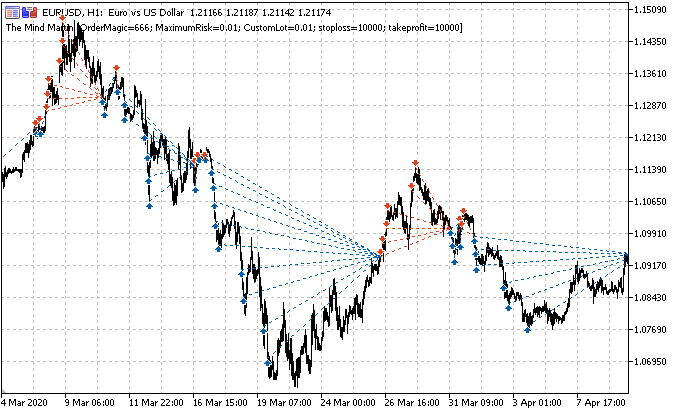
The main task is to correctly label the deals. Let us remember how this was done for single positions in previous articles. We set a random or deterministic horizon of deals, for example, 15 bars. If the market was rising in these 15 bars, the deal was labeled as Buying, otherwise it was Selling. A similar logic is used for a grid of orders, but here it is necessary to take into account the total profit/loss for a group of open positions. This can be illustrated with a simple example. The author tried his best to draw the image.

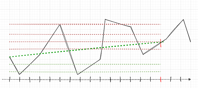
Suppose that the deal horizon is 15 (fifteen) bars (marked with a vertical red stroke on the conventional time scale). If a single position is used, it will be labeled as Buy (oblique green dash-dotted line), since the market has grown from one point to another. The market here is shown as a black broken curve.

With such labeling, intermediate market fluctuations are ignored. If we apply a grid of orders (red and green horizontal lines), then it is necessary to calculate the total profit for all triggered pending orders including the order opened at the very beginning (you can open a position and place the grid in the same direction, or optionally a grid of pending orders can be placed immediately, without opening a position). Such labeling will continue in a sliding window, for the entire depth of the learning history. The task of ML (machine learning) is to generalize the whole variety of situations and to efficiently predict on new data (if possible).

In this case, there may be several options for selecting the trade direction and for labeling the data. The choice task here is both philosophical and experimental.

• Selection by the maximum total profit. If a Sell grid generates more profit, this grid is labeled.
• Weighted choice between the number of open orders and the total profit. If the average profit for each open order in the grid is higher than that for the opposite side, then this side is selected.
• Selection by the maximum number of triggered orders. Since the desired robot should trade the grid, this option looks reasonable. If the number of triggered orders is maximum and the total position is in profit, then this side is selected. The side here means the direction of the grid (sell or buy).

These three criteria seem enough for the beginning. Let us consider in detail the first one, since it is the simplest one and is aimed at maximum profit.

Labeling Deals in Code

Let us now recall how deals were labeled in the previous articles.

def add_labels(dataset, min, max):
    labels = []
    for i in range(dataset.shape[0]-max):
        rand = random.randint(min, max)
        curr_pr = dataset['close'][i]
        future_pr = dataset['close'][i + rand]
        
        if future_pr + MARKUP < curr_pr:
            labels.append(1.0)
        elif future_pr - MARKUP > curr_pr:
            labels.append(0.0)
        else:
            labels.append(2.0)
    dataset = dataset.iloc[:len(labels)].copy()
    dataset['labels'] = labels
    dataset = dataset.dropna()
    dataset = dataset.drop(
        dataset[dataset.labels == 2].index).reset_index(drop=True)
    return dataset

This code needs to be generalized for a regular grid and a martingale grid. Another exciting feature is that you can explore grids with different numbers of orders, with different distances between orders, and even apply martingale (lot increase).

To do this, let us add global variables which later can be used and optimized.

GRID_SIZE = 10
GRID_DISTANCES = np.full(GRID_SIZE, 0.00200)
GRID_COEFFICIENTS = np.linspace(1, 3, num= GRID_SIZE)

The GRID_SIZE variable contains the number if orders in both directions.

GRID_DISTANCES sets the distance between orders. The distance can be fixed or variable (different for all orders). This will help increase the trading system flexibility.

The GRID_COEFFICIENTS variable contains lot multiplier for each order. If they are constant, the system will create a regular grid. If the lots are different, then it will be martingale or anti-martingale, or any other name applicable to a grid with different lot multipliers.

For those of you who are new to the numpy library:

• np.full fills an array with a specified number of identical values
• np.linspace fills an array with the specified number of the values which are evenly distributed between two real numbers. In the above example, GRID_COEFFICIENTS will contain the following.

array([1.        , 1.22222222, 1.44444444, 1.66666667, 1.88888889,
       2.11111111, 2.33333333, 2.55555556, 2.77777778, 3.        ])

Accordingly, the first lot multiplier will be equal to one, so this lot will be equal to the basic lot specified in the trading system parameters. Multipliers from 1 to 3 will be used successively for further grid orders. In order to use this grid with a fixed multiplier for all orders, call np.full. 

Accounting for triggered and not triggered orders can be somewhat tricky, and thus we need to create some kind of data structure. I decided to create a dictionary for keeping records of orders and positions for each specific case (sample). Instead, we could use a Data Class object, a pandas Data Frame, or a numpy structured array. The last solution, perhaps, would be the fastest, but here it is not critical.

A dictionary storing information about an order grid will be created at each iteration of adding a sample to the training set. This may need some explanation. The grid_stats dictionary contains all the required information about the current order grid from its opening to closing. 

def add_labels(dataset, min, max, distances, coefficients):
    labels = []
    for i in range(dataset.shape[0]-max):
        rand = random.randint(min, max)
        all_pr = dataset['close'][i:i + rand + 1]

        grid_stats = {'up_range': all_pr[0] - all_pr.min(),
                      'dwn_range': all_pr.max() - all_pr[0],
                      'up_state': 0,
                      'dwn_state': 0,
                      'up_orders': 0,
                      'dwn_orders': 0,
                      'up_profit': all_pr[-1] - all_pr[0] - MARKUP,
                      'dwn_profit': all_pr[0] - all_pr[-1] - MARKUP
                      }

        for i in np.nditer(distances):
            if grid_stats['up_state'] + i <= grid_stats['up_range']:
                grid_stats['up_state'] += i
                grid_stats['up_orders'] += 1
                grid_stats['up_profit'] += (all_pr[-1] - all_pr[0] + grid_stats['up_state']) \
                * coefficients[int(grid_stats['up_orders']-1)]
                grid_stats['up_profit'] -= MARKUP * coefficients[int(grid_stats['up_orders']-1)]

            if grid_stats['dwn_state'] + i <= grid_stats['dwn_range']:
                grid_stats['dwn_state'] += i
                grid_stats['dwn_orders'] += 1
                grid_stats['dwn_profit'] += (all_pr[0] - all_pr[-1] + grid_stats['dwn_state']) \
                * coefficients[int(grid_stats['dwn_orders']-1)]
                grid_stats['dwn_profit'] -= MARKUP * coefficients[int(grid_stats['dwn_orders']-1)]
        
        if grid_stats['up_profit'] > grid_stats['dwn_profit'] and grid_stats['up_profit'] > 0:
            labels.append(0.0)
            continue
        elif grid_stats['dwn_profit'] > 0:
            labels.append(1.0)
            continue
        
        labels.append(2.0)

    dataset = dataset.iloc[:len(labels)].copy()
    dataset['labels'] = labels
    dataset = dataset.dropna()
    dataset = dataset.drop(
        dataset[dataset.labels == 2].index).reset_index(drop=True)
    return dataset

The all_pr variable contains prices, from the current to a future one. It is needed to calculate the grid itself. To build the grid, we want to know the price ranges from the first bar to the last one. These values are contained in the 'up_range' and 'dwn_range' dictionary entries. Variables 'up_profit' and 'dwn_profit' will contain the final profit from the use of the Buy or Sell grid on the current history segment. These values are initialized with the profit received from one market deal, which was opened initially. Then they will be summed with the deals which were opened according to the grid if pending orders triggered.

Now we need to loop through all GRID_DISTANCES and to check if the pending limit orders have triggered. If an order is in the range of up_range or dwn_range, then the order has triggered. In this case we increment the appropriate up_state and dwn_state counters which store the level of the last activated order. At the next iteration, the distance to the new order in the grid is added to this level - if this order is in the price range, then it has also triggered.

Additional information is written for all triggered orders. For example, the profit of a pending order is added to the total value. For buy positions, this profit is calculated using the following formula. Here the position open price is subtracted from the last price (at which the position is supposed to close), the distance to the selected pending order from the series is added and the result is multiplied by the lot multiplier for this order in the grid. An opposite calculation is used for sell orders. The accumulated markup is additionally calculated. 

grid_stats['up_profit'] += (all_pr[-1] - all_pr[0] + grid_stats['up_state']) \
                * coefficients[int(grid_stats['up_orders']-1)]
grid_stats['up_profit'] -= MARKUP * coefficients[int(grid_stats['up_orders']-1)]

The next block of code checks the profit for Buy and Sell grids. If the profit, taking into account the accumulated markups, is greater than zero and is maximal, then the corresponding sample is added to the training set. If none of the conditions are met, the 2.0 mark is added - the samples marked with this mark are removed from the training dataset as they are considered uninformative. These conditions can be changed later, depending on the desired grid building options.

Upgrading the Tester to Work with the Order Grid 

To correctly calculate the profit gained from trading the grid, we need to modify the strategy tester. I decided to make it similar to the MetaTrader 5 Tester, so that it sequentially loops through the history of quotes and opens and closes trades as if it were a real trade. This improves code understanding and avoids peeking into the future. I will focus on the main points of the code. I will not provide the old tester version here, but you can find it in my previous articles. I suppose that some readers will not understand the code below, as they would like to quickly get hold of the Grail, without going into any details. However, the key points should be clarified.

def tester(dataset, markup, distances, coefficients, plot=False):
    last_deal = int(2)
    all_pr = np.array([])
    report = [0.0]
    for i in range(dataset.shape[0]):
        pred = dataset['labels'][i]
        all_pr = np.append(all_pr, dataset['close'][i])

        if last_deal == 2:
            last_deal = 0 if pred <= 0.5 else 1
            continue

        if last_deal == 0 and pred > 0.5:
            last_deal = 1
            up_range = all_pr[0] - all_pr.min()
            up_state = 0
            up_orders = 0
            up_profit = (all_pr[-1] - all_pr[0]) - markup
            report.append(report[-1] + up_profit)
            up_profit = 0
            for d in np.nditer(distances):
                if up_state + d <= up_range:
                    up_state += d
                    up_orders += 1
                    up_profit += (all_pr[-1] - all_pr[0] + up_state) \
                    * coefficients[int(up_orders-1)]
                    up_profit -= markup * coefficients[int(up_orders-1)]    
                    report.append(report[-1] + up_profit)
                    up_profit = 0
            all_pr = np.array([dataset['close'][i]])
            continue

        if last_deal == 1 and pred < 0.5:
            last_deal = 0
            dwn_range = all_pr.max() - all_pr[0]
            dwn_state = 0
            dwn_orders = 0
            dwn_profit = (all_pr[0] - all_pr[-1]) - markup
            report.append(report[-1] + dwn_profit)
            dwn_profit = 0
            for d in np.nditer(distances):
                if dwn_state + d <= dwn_range:
                    dwn_state += d
                    dwn_orders += 1
                    dwn_profit += (all_pr[0] + dwn_state - all_pr[-1]) \
                    * coefficients[int(dwn_orders-1)]
                    dwn_profit -= markup * coefficients[int(dwn_orders-1)] 
                    report.append(report[-1] + dwn_profit)
                    dwn_profit = 0
            all_pr = np.array([dataset['close'][i]])   
            continue

    y = np.array(report).reshape(-1, 1)
    X = np.arange(len(report)).reshape(-1, 1)
    lr = LinearRegression()
    lr.fit(X, y)

    l = lr.coef_
    if l >= 0:
        l = 1
    else:
        l = -1

    if(plot):
        plt.figure(figsize=(12,7))
        plt.plot(report)
        plt.plot(lr.predict(X))
        plt.title("Strategy performance")
        plt.xlabel("the number of trades")
        plt.ylabel("cumulative profit in pips")
        plt.show()

    return lr.score(X, y) * l

Historically, grid traders are only interested in the balance curve, while they ignore the equity curve. So, we will adhere to this tradition and will not overcomplicate our complex tester. We will only display the balance graph. Furthermore, the equity curve can always be viewed in the MetaTrader 5 terminal. 

We loop through all prices and add them to the all_pr array. Further there are three options marked above. Since this tester was considered in previous articles, I will only explain the options for closing the order grid when an opposite signal appears. Just like when labeling the deals, the up_range variable stores the range of iterated prices by the time of closing open positions. Next, the profit of the first position (opened by market) is calculated. Then, the cycle checks for the presence of triggered pending orders. If there are any, their result is added to the balance graph. The same is performed for Sell orders/positions. Thus, the balance graph reflects all closed positions, and not the total profit by group. 

Testing New Methods for Working with Order Grids

Data preparation for machine learning is already familiar to us. First obtain prices and a set of features, then label the data (create Buy and Sell labels), and then check the labeling in the custom tester.

# Get prices and labels and test it

pr = get_prices(START_DATE, END_DATE)
pr = add_labels(pr, 15, 15, GRID_DISTANCES, GRID_COEFFICIENTS)
tester(pr, MARKUP, GRID_DISTANCES, GRID_COEFFICIENTS, plot=True)

Now we need to train the CatBoost model and test it on new data. I decided to use training on synthetic data generated by the Gaussian mixture model again, as it works well.

# Learn and test CatBoost model

gmm = mixture.GaussianMixture(
    n_components=N_COMPONENTS, covariance_type='full', n_init=1).fit(pr[pr.columns[1:]])
res = []
for i in range(10):
    res.append(brute_force(10000))
    print('Iteration: ', i, 'R^2: ', res[-1][0])
res.sort()
test_model(res[-1])

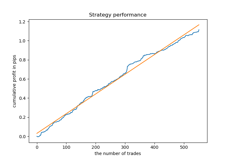
In this example, we will train ten models on 10,000 generated samples and choose the best one through an R^2 score. The learning process is as follows.

Iteration:  0 R^2:  0.8719436661855786
Iteration:  1 R^2:  0.912006346274096
Iteration:  2 R^2:  0.9532278725035132
Iteration:  3 R^2:  0.900845571741786
Iteration:  4 R^2:  0.9651728908727953
Iteration:  5 R^2:  0.966531822300101
Iteration:  6 R^2:  0.9688263099200539
Iteration:  7 R^2:  0.8789927823514787
Iteration:  8 R^2:  0.6084261786804662
Iteration:  9 R^2:  0.884741078512629

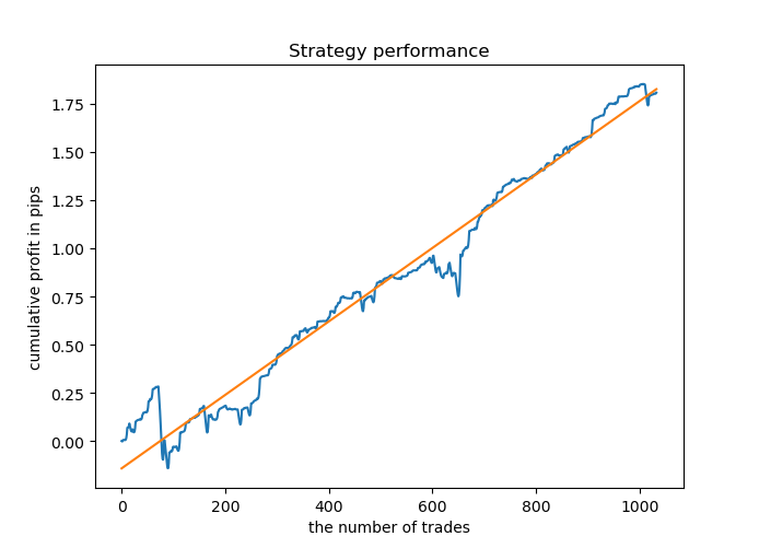
Most of the models have a high R^2 score on new data, which indicates a high stability of the model. Here is the resulting balance graph on training data and on data outside training.

Looks good. Now we can export the trained model in MetaTrader 5 and check its result in the terminal tester. Before testing, it is necessary to prepare the trading Expert Advisor and the include file. Each trained model will have its own file, so it is easy to store and change them.

Exporting the CatBoost Model to MQL5

Call the following function to export the model.

export_model_to_MQL_code(res[-1][1])

The function has been slightly modified. The explanation of this modification follows below.

def export_model_to_MQL_code(model):
    model.save_model('catmodel.h',
                     format="cpp",
                     export_parameters=None,
                     pool=None)

    # add variables
    code = '#include <Math\Stat\Math.mqh>'
    code += '\n'
    code += 'int MAs[' + str(len(MA_PERIODS)) + \
        '] = {' + ','.join(map(str, MA_PERIODS)) + '};'
    code += '\n'
    code += 'int grid_size = ' + str(GRID_SIZE) + ';'
    code += '\n'
    code += 'double grid_distances[' + str(len(GRID_DISTANCES)) + \
        '] = {' + ','.join(map(str, GRID_DISTANCES)) + '};'
    code += '\n'
    code += 'double grid_coefficients[' + str(len(GRID_COEFFICIENTS)) + \
        '] = {' + ','.join(map(str, GRID_COEFFICIENTS)) + '};'
    code += '\n'

    # get features
    code += 'void fill_arays( double &features[]) {\n'
    code += '   double pr[], ret[];\n'
    code += '   ArrayResize(ret, 1);\n'
    code += '   for(int i=ArraySize(MAs)-1; i>=0; i--) {\n'
    code += '       CopyClose(NULL,PERIOD_CURRENT,1,MAs[i],pr);\n'
    code += '       double mean = MathMean(pr);\n'
    code += '       ret[0] = pr[MAs[i]-1] - mean;\n'
    code += '       ArrayInsert(features, ret, ArraySize(features), 0, WHOLE_ARRAY); }\n'
    code += '   ArraySetAsSeries(features, true);\n'
    code += '}\n\n'

    # add CatBosst
    code += 'double catboost_model' + '(const double &features[]) { \n'
    code += '    '
    with open('catmodel.h', 'r') as file:
        data = file.read()
        code += data[data.find("unsigned int TreeDepth")
                               :data.find("double Scale = 1;")]
    code += '\n\n'
    code += 'return ' + \
        'ApplyCatboostModel(features, TreeDepth, TreeSplits , BorderCounts, Borders, LeafValues); } \n\n'

    code += 'double ApplyCatboostModel(const double &features[],uint &TreeDepth_[],uint &TreeSplits_[],uint &BorderCounts_[],float &Borders_[],double &LeafValues_[]) {\n\
    uint FloatFeatureCount=ArrayRange(BorderCounts_,0);\n\
    uint BinaryFeatureCount=ArrayRange(Borders_,0);\n\
    uint TreeCount=ArrayRange(TreeDepth_,0);\n\
    bool     binaryFeatures[];\n\
    ArrayResize(binaryFeatures,BinaryFeatureCount);\n\
    uint binFeatureIndex=0;\n\
    for(uint i=0; i<FloatFeatureCount; i++) {\n\
       for(uint j=0; j<BorderCounts_[i]; j++) {\n\
          binaryFeatures[binFeatureIndex]=features[i]>Borders_[binFeatureIndex];\n\
          binFeatureIndex++;\n\
       }\n\
    }\n\
    double result=0.0;\n\
    uint treeSplitsPtr=0;\n\
    uint leafValuesForCurrentTreePtr=0;\n\
    for(uint treeId=0; treeId<TreeCount; treeId++) {\n\
       uint currentTreeDepth=TreeDepth_[treeId];\n\
       uint index=0;\n\
       for(uint depth=0; depth<currentTreeDepth; depth++) {\n\
          index|=(binaryFeatures[TreeSplits_[treeSplitsPtr+depth]]<<depth);\n\
       }\n\
       result+=LeafValues_[leafValuesForCurrentTreePtr+index];\n\
       treeSplitsPtr+=currentTreeDepth;\n\
       leafValuesForCurrentTreePtr+=(1<<currentTreeDepth);\n\
    }\n\
    return 1.0/(1.0+MathPow(M_E,-result));\n\
    }'

    file = open('C:/Users/dmitrievsky/AppData/Roaming/MetaQuotes/Terminal/D0E8209F77C8CF37AD8BF550E51FF075/MQL5/Include/' +
                str(SYMBOL) + '_cat_model_martin' + '.mqh', "w")
    file.write(code)
    file.close()
    print('The file ' + 'cat_model' + '.mqh ' + 'has been written to disc')

The grid settings that were used during training are now saved. They will also be used in trading. 

The Moving Average from the standard terminal pack and indicator buffers are no longer used. Instead, all features are calculated in the function body. When adding original features, such features also should be added to the export function.

Green highlights the path to the Include folder of your terminal. It allows saving the .mqh file and connecting it to the Expert Advisor.

Let us view the .mqh file itself (the CatBoost model is omitted here)

#include <Math\Stat\Math.mqh>
int MAs[14] = {5,25,55,75,100,125,150,200,250,300,350,400,450,500};
int grid_size = 10;
double grid_distances[10] = {0.003,0.0035555555555555557,0.004111111111111111,0.004666666666666666,0.005222222222222222,
			     0.0057777777777777775,0.006333333333333333,0.006888888888888889,0.0074444444444444445,0.008};
double grid_coefficients[10] = {1.0,1.4444444444444444,1.8888888888888888,2.333333333333333,
				2.7777777777777777,3.2222222222222223,3.6666666666666665,4.111111111111111,4.555555555555555,5.0};
void fill_arays( double &features[]) {
   double pr[], ret[];
   ArrayResize(ret, 1);
   for(int i=ArraySize(MAs)-1; i>=0; i--) {
       CopyClose(NULL,PERIOD_CURRENT,1,MAs[i],pr);
       double mean = MathMean(pr);
       ret[0] = pr[MAs[i]-1] - mean;
       ArrayInsert(features, ret, ArraySize(features), 0, WHOLE_ARRAY); }
   ArraySetAsSeries(features, true);
}

As you can see, all the grid settings have been saved and the model is ready to work. You only need to connect it to the Expert Advisor.

#include <EURUSD_cat_model_martin.mqh>

Now I would like to explain the logic according to which the Expert Advisor processes signals. The OnTick() function is used as an example. The bot uses the MT4Orders library which should be additionally downloaded.

void OnTick() {
//---
   if(!isNewBar()) return;
   TimeToStruct(TimeCurrent(), hours);
   double features[];

   fill_arays(features);
   if(ArraySize(features) !=ArraySize(MAs)) {
      Print("No history available, will try again on next signal!");
      return;
   }
   double sig = catboost_model(features);

// Close positions by an opposite signal
   if(count_market_orders(0) || count_market_orders(1))
      for(int b = OrdersTotal() - 1; b >= 0; b--)
         if(OrderSelect(b, SELECT_BY_POS) == true) {
            if(OrderType() == 0 && OrderSymbol() == _Symbol && OrderMagicNumber() == OrderMagic && sig > 0.5)
               if(OrderClose(OrderTicket(), OrderLots(), OrderClosePrice(), 0, Red)) {
               }
            if(OrderType() == 1 && OrderSymbol() == _Symbol && OrderMagicNumber() == OrderMagic && sig < 0.5)
               if(OrderClose(OrderTicket(), OrderLots(), OrderClosePrice(), 0, Red)) {
               }
         }

// Delete all pending orders if there are no pending orders
   if(!count_market_orders(0) && !count_market_orders(1)) {

      for(int b = OrdersTotal() - 1; b >= 0; b--)
         if(OrderSelect(b, SELECT_BY_POS) == true) {

            if(OrderType() == 2 && OrderSymbol() == _Symbol && OrderMagicNumber() == OrderMagic )
               if(OrderDelete(OrderTicket())) {
               }

            if(OrderType() == 3 && OrderSymbol() == _Symbol && OrderMagicNumber() == OrderMagic )
               if(OrderDelete(OrderTicket())) {
               }
         }
   }

// Open positions and pending orders by signals
   if(countOrders() == 0 && CheckMoneyForTrade(_Symbol,LotsOptimized(),ORDER_TYPE_BUY)) {
      double l = LotsOptimized();

      if(sig < 0.5) {
         OrderSend(Symbol(),OP_BUY,l, Ask, 0, Bid-stoploss*_Point, Ask+takeprofit*_Point, NULL, OrderMagic);
         double p = Ask;
         for(int i=0; i<grid_size; i++) {
            p = NormalizeDouble(p - grid_distances[i], _Digits);
            double gl = NormalizeDouble(l * grid_coefficients[i], 2);
            OrderSend(Symbol(),OP_BUYLIMIT,gl, p, 0, p-stoploss*_Point, p+takeprofit*_Point, NULL, OrderMagic);
         }
      }
      else {
         OrderSend(Symbol(),OP_SELL,l, Bid, 0, Ask+stoploss*_Point, Bid-takeprofit*_Point, NULL, OrderMagic);
         double p = Ask;
         for(int i=0; i<grid_size; i++) {
            p = NormalizeDouble(p + grid_distances[i], _Digits);
            double gl = NormalizeDouble(l * grid_coefficients[i], 2);
            OrderSend(Symbol(),OP_SELLLIMIT,gl, p, 0, p+stoploss*_Point, p-takeprofit*_Point, NULL, OrderMagic);
         }
      }
   }
}

The fill_arrays function prepares features for the CatBoost model filling the features array. Then this array is passed to the catboost_model() function, which returns a signal in the range of 0;1.

As you can see from the example of Buy orders, the grid_size variable is used here. It shows the number of pending orders, which are located at a distance of grid_distances. The standard lot is multiplied by the coefficient from the grid_coefficients array, which corresponds to the order number.

After the bot is compiled, we can proceed to testing.

Checking the bot in the MetaTrader 5 Tester

Testing should be performed on the timeframe on which the bot was trained. In this case it is H1. It can be tested using open prices, since the bot has an explicit control of bar opening. However, since a grid is used, M1 OHLC can be selected for greater accuracy.

This particular bot was trained in the following period:

START_DATE = datetime(2020, 5, 1)
TSTART_DATE = datetime(2019, 1, 1)
FULL_DATE = datetime(2018, 1, 1)
END_DATE = datetime(2022, 1, 1)

• The interval from the fifth month of 2020 to the present day is a training period, which is divided 50/50 into training and validation subsamples. 
• From the 1st month of 2019, the model was evaluated according to R^2 and the best one was chosen.
• From the 1st month of 2018, the model was tested in a custom tester.
• Synthetic data was used for training (generated by the Gaussian mixture model)
• The CatBoost model has a strong regularization which helps to avoid overfitting on the training sample.

All these factors indicate (which is also confirmed by the custom tester) that we have found a certain pattern in the interval from 2018 to the present day.

Lest us view how it looks like in the MetaTrader 5 Strategy Tester.

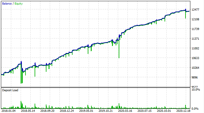
With the exception that we can now see equity drawdowns, the balance chart looks the same as in my custom tester. It is good news. Let us make sure that the bot is trading exactly the grid and nothing else.

Here is the testing result at the interval from 2015.

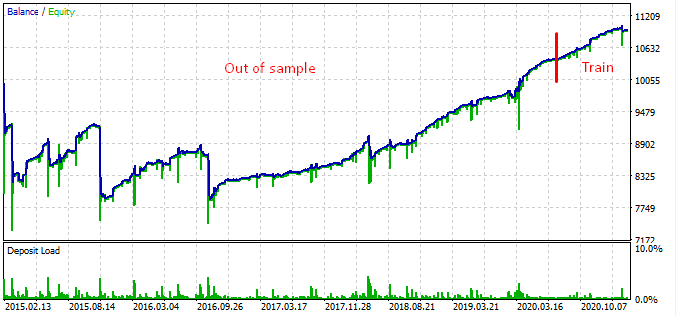
According to the graph, the found pattern works from the end of 2016 to the present day, in the rest interval it fails. In this case the initial lot is minimal, which helped the bot to survive. At least we know that the bot is effective since the beginning of 2017. Based on this, we can increase the risk in an effort to increase the profitability. The robot shows impressive results: 1600% in 3 years with a drawdown of 40%, having a hypothetical risk to lose the entire deposit.

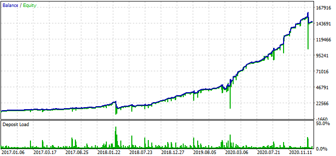
Also, the bot uses Stop Loss and Take Profit for each position. SL and TP can be used while sacrificing performance but limiting risks. 

Please note that I used quite an aggressive grid.

GRID_COEFFICIENTS = np.linspace(1, 5, num= GRID_SIZE)

array([1.        , 1.44444444, 1.88888889, 2.33333333, 2.77777778,
       3.22222222, 3.66666667, 4.11111111, 4.55555556, 5.        ])

The last multiplier is equal to five. This means that the lot of the last order in the series is five times higher than the initial lot, which entails additional risks. You can choose more moderate modes.

Why did the bot stop working in the period from 2016 and earlier? I have no meaningful answer to this question. It seems that there are long seven-year cycles in the Forex market or shorter ones, the patterns of which are in no way connected with each other. This is a separate topic, which requires a more detailed research.

Conclusion

In this article, I tried to describe the technique which can be used to train a boosting model or a neural network to trade martingale. The article features a ready-made solution, with which you can create your own trading robots.