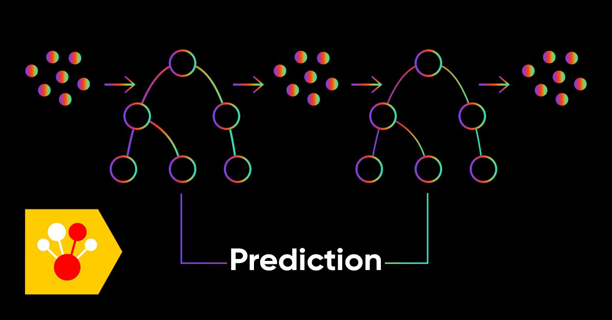
Gradient boosting in transductive and active machine learning

Introduction

Semi-supervised  or transductive learning uses unlabeled data allowing the model to better understand the general data structure. This is similar to our thinking. By remembering only a few images, the human brain is able to extrapolate knowledge about these images to new objects in general terms, without focusing on insignificant details. This results in less overfitting and in better generalization. 

Transduction was introduced by Vladimir Vapnik, who is the co-inventor of the Support-Vector Machine (SVM). He believes that the transduction is preferable to induction since induction requires solving a more general problem (inferring a function) before solving a more specific problem (computing outputs for new cases). 

 "When solving a problem of interest, do not solve a more general problem as an intermediate step. Try to get the answer that you really need but not a more general one." 

This Vapnik's assumption is similar to the observation which had been made earlier by Bertrand Russell:

"we shall reach the conclusion that Socrates is mortal with a greater approach to certainty if we make our argument purely inductive than if we go by way of 'all men are mortal' and then use deduction".

Unsupervised learning (with unlabeled data) is expected to become much more important in the long run. Unsupervised learning is usually typical of people and animals: they discover the structure of the world by observing, not by recognizing the name of each object. 

Thus, semi-supervised learning combines both processes: supervised learning occurs on a small amount of labeled data, after which the model extrapolates its knowledge to a large unlabeled area. 

The use of unlabeled data implies some connection with the underlying data distribution. At least one of the following assumptions must be met:

• Continuity assumption. Points that are close to each other are more likely to share a label. This is also assumed in supervised learning and yields a preference for geometrically simple boundaries that separate classes. In the case of semi-supervised learning, the smoothness assumption additionally yields a preference in low-density regions, where few points are close to each other but in different classes.
• Cluster assumption. The data tends to form discrete clusters, and points in the same cluster are more likely to share a label (although data that shares a label can spread across multiple clusters). This is a special case of the smoothness assumption that leads to learning with clustering algorithms.
  
• Manifold assumption. The data lies approximately on a manifold of much lower dimension than the input space. In this case, learning the manifold using both the labeled and unlabeled data can avoid the curse of dimensionality. Then learning can continue using distances and densities defined on the manifold.
  

Check the link for more details about semi-controlled learning.

The main method on semi-supervised learning is pseudo-labeling which is implemented as follows:

• Some measure of proximity (for example, Euclidean distance) is used to label the rest of the data based on the labeled data region (pseudo-label).
• Training labels are combined with pseudo-labels and signs.
• The model is trained on the entire dataset.

According to the researchers, the use of labeled data in combination with unlabeled data can significantly improve the model accuracy. I used a similar idea in my previous article, in which I used the estimation of the probability density of the distribution of labeled data and sampling from this distribution. But the distribution of new data may be different, so semi-supervised learning can provide some benefits, as the experiment in this article will show.

Active learning is a certain logical continuation of semi-supervised learning. It is an iterative process of labeling new data in such a way that the boundaries separating the classes are optimally located.

The main hypothesis of active learning states that the learning algorithm can choose the data it wants to learn from. It can perform better than traditional methods with significantly less training data. Traditional methods here refer to conventional supervised learning using labeled data. Such training can be called passive. The model is simply trained on labeled data. The more data, the better. One of the most time-consuming problems in passive learning is data collection and labeling. In many cases, there can be restrictions associated with the collection of additional data or with their adequate labeling. 

Active learning has three most popular scenarios, in which the learning model will request new class instance labels from the unlabeled region:

• Membership query synthesis. In this case, the model generates an instance from a certain distribution which is common to all examples. This can be a class instance with added noise, or just a plausible point in the space in question. This new point is sent to the oracle for training. Oracle is the conventional name for an evaluator function that evaluates the value of a given feature instance for the model.
• Stream-based sampling. According to this scenario, each unlabeled data point is examined one at a time, after which the Oracle chooses whether it wants to query a class label for this point or to reject it based on some information criterion. 
• Pool-based sampling. In this scenario, there is a large pool of unlabeled examples, as in the previous case. Instances are selected from the pool based on informativeness. The most informative instances are selected from the pool. This is the most popular scenario among active learning fans. All unlabeled instances will be ranked, and then the most informative instances will be selected.

Each scenario can be based on a specific query strategy. As mentioned above, the main difference between active and passive learning is the ability to query instances from an unlabeled region based on past queries and model responses. Therefore, all queries require some measure of informativeness. 

The most popular query strategies are as follows:

• Uncertainty sampling (least confidence). According to this strategy, we select the instance for which the model is least certain. For example, the probability of assigning a label to a certain class is below a certain boundary.
• Margin sampling. The disadvantage of the first strategy is that it determines the probability of belonging to only one label, while disregarding the probabilities of belonging to other labels. The margin sampling strategy selects the smallest probability difference between the two most likely labels.
• Entropy sampling. The entropy formula is applied to each instance, and the instance with the highest value is queried.

Similar to semi-supervised learning, the active learning process consists of several steps:

• The model is trained on labeled data.
  
• The same model is used to label unlabeled data to predict probabilities (pseudo-labels).
• New instance query strategy is selected.
• N instances are selected from the data pool according to the informativeness and are added to the training sample. 
• This cycle is repeated until some stop criterion is reached. A stop criterion can be the number of iterations or the estimate of the learning error, as well as other external criteria.

Active Learning

Let us go straight to active learning and test its effectiveness on our data.

There are several libraries for active learning in the Python language, the most popular of them being:

• modAL is quite a simple and easy-to-learn package, which is a kind of a wrapper for the popular machine learning library scikit-learn (they are fully compatible). The package provides the most popular active learning methods.
• Libact uses the multi-armed bandit strategy over existing query strategies for a dynamic selection of the best query. 
• Alipy is a kind of a laboratory from package providers, which contains a large number of query strategies.

I have selected the modAL library as being more intuitive and suitable for getting acquainted with the active learning philosophy. It offers greater freedom in designing models and in creating your own models by using standard blocks or by creating your own ones.

Let us consider the above described process using the below scheme, which does not require further explanations:

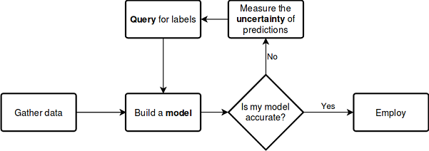
See the documentation

The great thing about the library is that you can use any scikit-learn classifier. The following example demonstrates the use of a random forest as a learning model:

from modAL.models import ActiveLearner
from modAL.uncertainty import entropy_sampling
from sklearn.ensemble import RandomForestClassifier

learner = ActiveLearner(
    estimator=RandomForestClassifier(),
    query_strategy=entropy_sampling,
    X_training=X_training, y_training=y_training
)

The random forest here acts as a learning model and as an evaluator allowing the selection of new samples from unlabeled data depending on the query strategy (for example, based on entropy, as in this example). Next, a dataset consisting of a small amount of labeled data is passed to the model. This is used for preliminary training. 

The modAL library enables an easy combination of query strategies and allows making composite weighted strategies out of them:

from modAL.utils.combination import make_linear_combination, make_product
from modAL.uncertainty import classifier_uncertainty, classifier_margin

# creating new utility measures by linear combination and product
# linear_combination will return 1.0*classifier_uncertainty + 1.0*classifier_margin
linear_combination = make_linear_combination(
    classifier_uncertainty, classifier_margin,
    weights=[1.0, 1.0]
)
# product will return (classifier_uncertainty**0.5)*(classifier_margin**0.1)
product = make_product(
    classifier_uncertainty, classifier_margin,
    exponents=[0.5, 0.1]
)

Once the query is generated, instances that meet the query criteria are selected from the unlabeled data region, using the multi_argmax or weighted_randm selectors:

from modAL.utils.selection import multi_argmax

# defining the custom query strategy, which uses the linear combination of
# classifier uncertainty and classifier margin
def custom_query_strategy(classifier, X, n_instances=1):
    utility = linear_combination(classifier, X)
    query_idx = multi_argmax(utility, n_instances=n_instances)
    return query_idx, X[query_idx]

custom_query_learner = ActiveLearner(
    estimator=GaussianProcessClassifier(1.0 * RBF(1.0)),
    query_strategy=custom_query_strategy,
    X_training=X_training, y_training=y_training
)

Query Strategies

There are three main query strategies. All strategies are based on classification uncertainty, which is why they are called uncertainty measures. Let us view how they work.

Classification uncertainty, in a simple case, is evaluated as U(x)=1−P(x^|x), where x is the case to be predicted, while x^ is the most probable forecast. For example, if there are three classes and three sample items, the corresponding uncertainties can be calculated as follows:

[[0.1 , 0.85, 0.05],
 [0.6 , 0.3 , 0.1 ],
 [0.39, 0.61, 0.0 ]]

1 - proba.max(axis=1)

[0.15, 0.4 , 0.39]

Thus, the second example will be selected as the most uncertain one.

Classification margin is the difference in the probabilities of the first and second most probable queries. The difference is determined according to the following formula: M(x)=P(x1^|x)−P(x2^|x), where x1^ and x2^ are the first and second most probable classes.

This query strategy selects instances with the smallest margin between the probabilities of the two most probable classes, because the smaller the margin of the solution, the more uncertain it is.

>>> import numpy as np
>>> proba = np.array([[0.1 , 0.85, 0.05],
...                   [0.6 , 0.3 , 0.1 ],
...                   [0.39, 0.61, 0.0 ]])
>>>
>>> proba
array([[0.1 , 0.85, 0.05],
       [0.6 , 0.3 , 0.1 ],
       [0.39, 0.61, 0.  ]])
>>> part = np.partition(-proba, 1, axis=1)
>>> part
array([[-0.85, -0.1 , -0.05],
       [-0.6 , -0.3 , -0.1 ],
       [-0.61, -0.39, -0.  ]])
>>> part[:, 0]
array([-0.85, -0.6 , -0.61])
>>> part[:, 1]
array([-0.1 , -0.3 , -0.39])
>>> margin = - part[:, 0] + part[:, 1]
>>> margin
array([0.75, 0.3 , 0.22])

In this case, the third sample (the third row of the array) will be selected, since the probability margin for this instance is minimal.

Classification entropy is calculated using the information entropy formula: H(x)=−∑kpklog(pk), where pk is the probability that the sample belongs to the k-th class. The closer the distribution is to uniform, the higher the entropy. In our example, the maximum entropy is obtained for the 2nd example.

[0.51818621, 0.89794572, 0.66874809]

It does not look very difficult. This description seems enough for understanding the three main query strategies. For further details please study the package documentation, because I only provide the basic points.

Batch query strategies

Querying one element at a time and retraining the model is not always efficient. A more efficient solution is to label and select multiple instances from the unlabeled data at once. There are a number of queries for this. The most popular of them is Ranked Set Sampling based on a similarity function such as cosine distance. This method estimates how well the feature space is explored near x (unlabeled instance). After evaluation, the instance with the highest rank is added to the training set and is removed from the unlabeled data pool. After that the rank is recalculated and the best instance is added again until the number of instances reaches the specified size (batch size). 

Information density queries

The simple query strategies described above do not evaluate the data structure. This can lead to sub-optimal queries. To improve sampling, you can use information density measures that will assist in correctly selecting the elements of unlabeled data. It uses cosine or Euclidean distance. The higher the information density, the more this selected instance is similar to all the others. 

Classification committee queries

This query type eliminates some of the disadvantages of simple query types. For example, the selection of elements tends to be biased due to the characteristics of a particular classifier. Some important sampling elements may be missing. This effect is eliminated by simultaneously storing several hypotheses and selecting queries between which there are disagreements. Thus, the committee of classifiers learns each on its own copy of the sample, and then the results are weighed. Other types of classifier committee learning include bagging and bootstrapping.

This short description almost completely covers the library functionality. You can refer to the documentation for further details.

Learning Actively

I have selected the batch query strategy, as well as the classifier committee queries, and ran a series of experiments. The batch query strategy did not show good performance on new data, however, by submitting the dataset it generated to GMM, I started to get interesting results. 

Consider an example of implementing the batch active learning function:

def active_learner(data, labeled_size, unlabeled_size, batch_size, max_depth):
    X_raw = data[data.columns[1:-1]].to_numpy()
    y_raw = data[data.columns[-1]].to_numpy()

    # Isolate our examples for our labeled dataset.
    training_indices = np.random.randint(low=0, high=X_raw.shape[0] + 1, size=labeled_size)

    X_train = X_raw[training_indices]
    y_train = y_raw[training_indices]

    # fit the model on all data
    cl = AdaBoostClassifier(DecisionTreeClassifier(max_depth=max_depth), n_estimators=50, learning_rate = 0.01)
    cl.fit(X_raw, y_raw)
    print('Score for the passive learning: ', cl.score(X_raw, y_raw), ' with train size: ', data.shape[0])

    # Isolate the non-training examples we'll be querying.
    X_pool = np.delete(X_raw, training_indices, axis=0)
    y_pool = np.delete(y_raw, training_indices, axis=0)

    # Pre-set our batch sampling to retrieve 3 samples at a time.
    preset_batch = partial(uncertainty_batch_sampling, n_instances=batch_size)

    # Specify our core estimator along with its active learning model.
    cl = AdaBoostClassifier(DecisionTreeClassifier(max_depth=3), n_estimators=50, learning_rate = 0.03)
    learner = ActiveLearner(estimator=cl, query_strategy=preset_batch, X_training=X_train, y_training=y_train)

The following is input to the function: a labeled dataset, the number of labeled instances, the number of unlabeled instances, the batch size for the batch label query and the maximum tree depth.

A specified number of labeled instances are randomly selected from the labeled dataset for model pre-training. The rest of the dataset forms a pool from which instances will be queried. I used AdaBoost as the basic classifier, which is similar to CatBoost. After that, the model is iteratively trained:

    # Allow our model to query our unlabeled dataset for the most
    # informative points according to our query strategy (uncertainty sampling).
    N_QUERIES = unlabeled_size // batch_size

    for index in range(N_QUERIES):
        query_index, query_instance = learner.query(X_pool)

        # Teach our ActiveLearner model the record it has requested.
        X, y = X_pool[query_index], y_pool[query_index]
        learner.teach(X=X, y=y)

        # Remove the queried instance from the unlabeled pool.
        X_pool, y_pool = np.delete(
            X_pool, query_index, axis=0), np.delete(y_pool, query_index)

        # Calculate and report our model's accuracy.
        model_accuracy = learner.score(X_raw, y_raw)
        print('Accuracy after query {n}: {acc:0.4f}'.format(
            n=index + 1, acc=model_accuracy))

        # Save our model's performance for plotting.
        performance_history.append(model_accuracy)

    print('Score for the active learning with train size: ',
          learner.X_training.shape)     

Since anything can happen as a result of such semi-supervised learning, the result can be any. However, after some manipulation with learner settings, I got the results comparable to those from the previous article. 

Ideally, the classification accuracy of an active learner on a small amount of labeled data should exceed the accuracy of a similar classifier with all data labeled.

>>> learned = active_learner(pr, 1000, 1000, 50)
Score for the passive learning:  0.5991245668429692  with train size:  5483
Accuracy after query 1: 0.5710
Accuracy after query 2: 0.5836
Accuracy after query 3: 0.5749
Accuracy after query 4: 0.5847
Accuracy after query 5: 0.5829
Accuracy after query 6: 0.5823
Accuracy after query 7: 0.5650
Accuracy after query 8: 0.5667
Accuracy after query 9: 0.5854
Accuracy after query 10: 0.5836
Accuracy after query 11: 0.5807
Accuracy after query 12: 0.5907
Accuracy after query 13: 0.5944
Accuracy after query 14: 0.5865
Accuracy after query 15: 0.5949
Accuracy after query 16: 0.5873
Accuracy after query 17: 0.5833
Accuracy after query 18: 0.5862
Accuracy after query 19: 0.5902
Accuracy after query 20: 0.6002
Score for the active learning with train size:  (2000, 8)

According to the report, the classifier which was trained on all labeled data, has an accuracy lower than that of the active learner which was trained by only 2000 instances. This is probably good. 

Now, this sample can be sent to the GMM model, after which the CatBoost classifier can be trained.

# prepare data for CatBoost
catboost_df = pd.DataFrame(learned.X_training)
catboost_df['labels'] = learned.y_training

# perform GMM clusterization over dataset
X = catboost_df.copy()
gmm = mixture.GaussianMixture(
    n_components=75, max_iter=500, covariance_type='full', n_init=1).fit(X)

# sample new dataset
generated = gmm.sample(10000)
# make labels
gen = pd.DataFrame(generated[0])
gen.rename(columns={gen.columns[-1]: "labels"}, inplace=True)
gen.loc[gen['labels'] >= 0.5, 'labels'] = 1
gen.loc[gen['labels'] < 0.5, 'labels'] = 0
X = gen[gen.columns[:-1]]
y = gen[gen.columns[-1]]
pr = pd.DataFrame(X)
pr['labels'] = y

# fit CatBoost model and test it
model = fit_model(pr)
test_model(model, TEST_START, END_DATE)

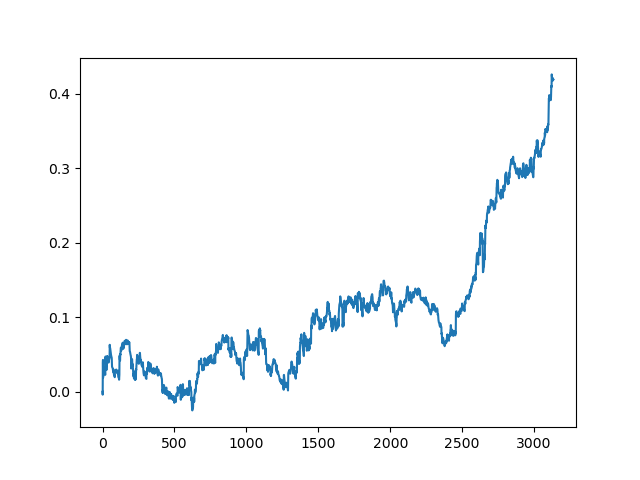
This process can be repeated several times, because at each stage of data processing there is an element of uncertainty which does not allow building unambiguous models. The following charts were obtained in the tester after all iterations (training period of 1 year followed by a 5-year testing period):

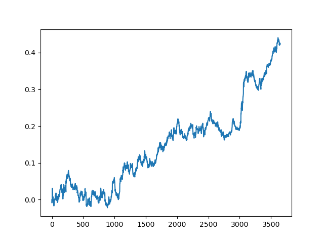
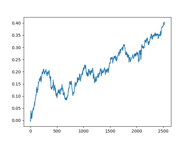
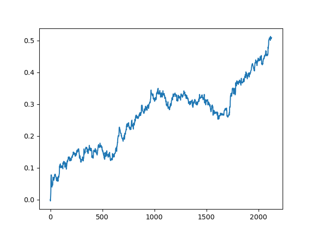
Of course, these results are not benchmark, and they only demonstrate that profitable (on new data) models can be obtained. 

Let us now implement the learning function on the classifier committee and see what happens:

def active_learner_committee(data, learners_number, labeled_size, unlabeled_size, batch_size):
    X_pool = data[data.columns[1:-1]].to_numpy()
    y_pool = data[data.columns[-1]].to_numpy()

    cl = AdaBoostClassifier(DecisionTreeClassifier(max_depth=3), n_estimators=50, learning_rate = 0.05)
    cl.fit(X_pool, y_pool)
    print('Score for the passive learning: ', cl.score(
        X_pool, y_pool), ' with train size: ', data.shape[0])

    # initializing Committee members
    learner_list = list()

    # Pre-set our batch sampling to retrieve 3 samples at a time.
    preset_batch = partial(uncertainty_batch_sampling, n_instances=batch_size)
    
    for member_idx in range(learners_number):
        # initial training data
        train_idx = np.random.choice(range(X_pool.shape[0]), size=labeled_size, replace=False)
        X_train = X_pool[train_idx]
        y_train = y_pool[train_idx]

        # creating a reduced copy of the data with the known instances removed
        X_pool = np.delete(X_pool, train_idx, axis=0)
        y_pool = np.delete(y_pool, train_idx)

        # initializing learner
        learner = ActiveLearner(
            estimator=AdaBoostClassifier(DecisionTreeClassifier(max_depth=2), n_estimators=50, learning_rate = 0.05),
            query_strategy=preset_batch,
            X_training=X_train, y_training=y_train
        )
        learner_list.append(learner)

    # assembling the committee
    committee = Committee(learner_list=learner_list)

    unqueried_score = committee.score(X_pool, y_pool)
    performance_history = [unqueried_score]

    N_QUERIES = unlabeled_size // batch_size

    for idx in range(N_QUERIES):
        query_idx, query_instance = committee.query(X_pool)
        committee.teach(
            X=X_pool[query_idx].reshape(1, -1),
            y=y_pool[query_idx].reshape(1, )
        )
        model_accuracy = committee.score(X_pool, y_pool)
        performance_history.append(model_accuracy)
        print('Accuracy after query {n}: {acc:0.4f}'.format(
            n=idx + 1, acc=model_accuracy))

        # remove queried instance from pool
        X_pool = np.delete(X_pool, query_idx, axis=0)
        y_pool = np.delete(y_pool, query_idx)

    return committee

Again, I have selected the batch query strategy to eliminate the need to retrain the model every time when one element is added. For the rest, I have created a committee of an arbitrary number of AdaBoost classifiers (I think it makes no sense to add more than five classifiers, but you can experiment). 

Below is a training score for a committee of five models with the same settings that were used for the previous method:

>>> committee = active_learner_committee(pr, 5, 1000, 1000, 50)
Score for the passive learning:  0.6533842794759825  with train size:  5496
Accuracy after query 1: 0.5927
Accuracy after query 2: 0.5818
Accuracy after query 3: 0.5668
Accuracy after query 4: 0.5862
Accuracy after query 5: 0.5874
Accuracy after query 6: 0.5906
Accuracy after query 7: 0.5918
Accuracy after query 8: 0.5910
Accuracy after query 9: 0.5820
Accuracy after query 10: 0.5934
Accuracy after query 11: 0.5864
Accuracy after query 12: 0.5753
Accuracy after query 13: 0.5868
Accuracy after query 14: 0.5921
Accuracy after query 15: 0.5809
Accuracy after query 16: 0.5842
Accuracy after query 17: 0.5833
Accuracy after query 18: 0.5783
Accuracy after query 19: 0.5732
Accuracy after query 20: 0.5828

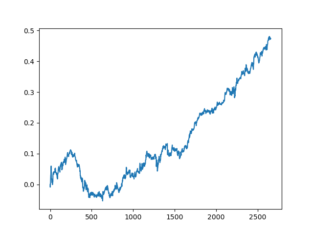
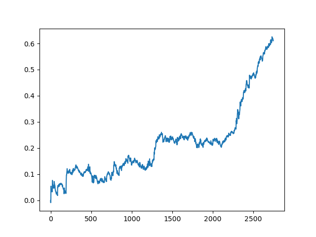
The results of the committee of active learners are not so good as those of one passive learner. It is impossible to guess the reasons. Perhaps this is just a random result. Then I ran the resulting dataset several times using the same principle and got the following random results:

Conclusions

In this article, we have considered active learning. The impression is unclear. On the one hand, it is always tempting to learn from a small number of instances, and these models do work well for some classification problems. However, this is still far from artificial intelligence. Such a model cannot find stable patterns among garbage data, and it requires more thorough preparation of features and labels, including data preparation based on expert labeling. I have not seen any significant increase in the quality of the models. At the same time, the labor intensity and time required to train the models has increased, which is a negative factor. I like the philosophy of active learning and the utilization of the features of human thinking. The attached file provides all the discussed functions. You can further explore these models and try to apply them in some other original way.