Combinatorics and probability theory for trading (Part I): The basics
Evgeniy Ilin | 31 August, 2021
Contents
- Introduction
- How can probability theory be useful in market analysis?
- Specifics of applied probability theory for manual and automated trading
- Probability trees and hypotheses
- About fractals
- Bernoulli scheme
- Creating the first fractal
- Summary
- Conclusion
Introduction
In my opinion, the language of probability theory can provide a completely different level of understanding of the processes running inside the market. Having understood the specifics of the probability theory, you will begin thinking in a completely new way. Vague ideas or some unproven tips will no longer cause the desire to hurry and trade on a real account. On the other hand, I understand that this new approach may not be comfortable for everyone. In this series, I want to show you a real and correct approach to trading. All decisions should be based on numbers only, and should avoid assumptions like "maybe", "what if", "it seems" and similar.
How can probability theory be useful in market analysis?
I have been involved technical science for quite a long period of my life, while the probability theory was the most difficult for me. This was because I didn't understand how wide its possibilities were. An indisputable advantage is its limitless capabilities, which depend only on your ingenuity and diligence, and of course your intelligence. After years spent on technical studying, I realized that the intelligence is not about the speed and attentiveness when performing the same types of operations, but it's about the flexibility of your mind. If we consider, for example, differential mathematics, the theory of vector and scalar fields, or even school algebra, they all imply a certain set of rules or recommendations, by following which you can solve almost any problem. Every non-standard task is a shock for our brain. In the theory of probability, there is an endless number of such moments — this is where many problems can be solved only by completely different approaches. In other words, intelligence can only be developed by diligence and willingness to solve a given problem, and the theory of probability can help you with this.
The framework of probability theory describes such fundamental trading concepts as mathematical expectation, possible probabilities of various events, averaged values, percentiles and more. Probability theory claims that there is no perfect trading system, and each system has its own risks. What we can do is only choose the trading system whose risks do not cause too much discomfort. What's more important is to correctly interpret these risks. In other words, we move from imprecise language of sensations or visual approximations to clear quantitative criteria. Of course, visual estimates are also important, but they work better when combined with quantitative variables. It is impossible to describe all the details and nuances in one article, but I will try to include some interesting information here. I hope you will find something useful here.
Specifics of applied probability theory for manual and automated trading
Before we proceed to using probability theory for market analysis, we first need to get acquainted with events and their probabilities. An event is a set of outcomes which meet some criteria, or which are grouped according to some criterion into a certain set. An outcome is a certain elementary element which is equal to every other element in the given group. The group refers to all the possible outcomes of a process. It is not so important what kind of process this is, what are its physics or how long the process takes. The important thing is that as a result of this process we will obtain something which had not existed before the process completed. Those outcomes that relate to our event, are essentially our event — for convenience, we combine them into a single object. The above idea can be visualized as follows:
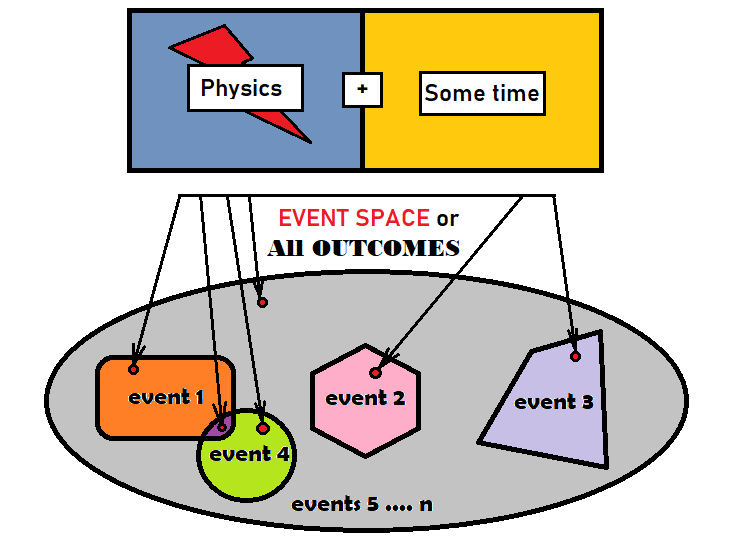
The gray ellipse in the above figure acts as all outcomes. In mathematics, it is called an event space. This does not mean that the event space has a geometric shape, but it is quite suitable for describing these concepts. There are 4 events inside the ellipse. As can be seen from the figure, there is a small red dot inside each event. There can be a limited or an unlimited number of such dots — it depends on the process under consideration. Two of the events in the figure intersect. Such events are referred to as the overlapping. So, there are some outcomes that belong to both events. All other events are non-overlapping as they are located in different parts of the ellipse and do not intersect geometrically. The rest of the gray area can be considered the last event, or it can also be broken down into smaller parts until there are no gray areas left.
Each event has at least one corresponding number which is usually called probability. Probability means how often this event would appear during repetitions of the same process if we could produce the same experiment indefinitely. There are two types of event spaces:
- With a finite number of possible outcomes
- With an infinite number of possible outcomes
If the number of outcomes is finite, the probability can be calculated as follows:
- P = S/N , S is the number of outcomes that meet the event criterion, N is the total number of all outcomes in the event space
In some cases, when the number of outcomes in a certain space is infinite, this probability can also be determined, for example using integrals. For the case in the image above, values "S" and "N" can be replaced by the areas of their geometric shapes.
It is not always possible to clearly define what the event space is, as well as to define the number of outcomes and the physics described by the events. These graphical representations should help our brain to analogize data so that instead of working not with some geometry, trying to understand what is going on, the brain could get used to the idea that we only work with probabilities and additional numbers that correspond to these probabilities. Events can also be referred to as states. If we use the logic of states, then the probability is exactly the frequency of emergence of a specific state as a result of repeating the same experiments.
By analogy with the areas of the figures, the sum of the areas of all figures included in the ellipse is exactly equal to the area of this ellipse. In terms of mathematics, the area is the number of outcomes that fall there. Hence:
- N = S[1] + S[2] + ... + S[n]
- S is the number of outcomes of a particular event
- N is all outcomes of the event space
By dividing both sides of the equality by the value N, we get an interesting and a very important relationship which underlies the whole theory of probability:
- 1 = S[1]/N + S[2]/N + ... +S[n]/N
Please note that this ratio only works for non-overlapping events. Because if events are joined, the shape areas overlap, and the sum of their areas will be greater than the area of the original ellipse. It is similar to a puzzle, in which the area of all puzzle pieces is exactly equal to the resulting image. In this case, a puzzle piece represents one of the events. All these fractions represent the probabilities of specific events:
- 1 = P[1] + P[2] + ... +P[n]
This ratio serves as the basis of the term collectively exhaustive event set. A collectively exhaustive event set is the unity of all non-overlapping events which form a certain space of events. For a puzzle, a collectively exhaustive set is all puzzle pieces. The total probability of all these events must be equal to one, which means that one of these events must necessarily occur as a result of the experiment. We don't know which event will occur, but we will find this out from the result of the experiment.
According to the above, any set of outcomes from the selected event space can serve as an event. This means that a collectively exhaustive set can be collected in all possible ways and combinations. When we deal with a finite number of outcomes, there may be a limited number of such combinations; for an infinite number of outcomes the number of combinations would always be infinite. If it is known that the number of outcomes equals infinity, mathematicians consider the concept of a random value. In some cases, random values can be more convenient to operate, as this is allowed by the task. A random value is a somewhat different method for describing the event space. In this case the outcome is the clear set of one or more numbers. We can say that this is a vector. This consideration model implies the concept of probability density.
These concepts will be used further, when exploring this topic, so let's consider them now. Probability density is a function that describes the entire event space. The dimension of this function is exactly equal to the number of numbers required to describe each outcome in this event space. For example, if we consider the problem of shooting at a target in a shooting range, the dimension of this function will be equal to two, because the target is flat (two-dimensional). In this case a particular outcome will be characterized by X and Y coordinates. These numbers are our random variables, so we can write the following:
- R = R(X,Y)
- R is the probability density of a bullet hitting a point with coordinates (X,Y)
The properties of this function are so that the full integral from minus to plus infinity for all variables of this function will be equal to one, which proves the above equation. The probabilities here are only determined by the integrals of that area in which the function is presented. Different events can be composed of piecewise integrated regions. So, it is possible to describe as many events as we need, because their number is infinite. This definition is enough within the framework of this article.
I'd like to add some more details about overlapping events. Such events are also very important for a general understanding of the picture as a whole. It is clear that with non-overlapping events should be easier to deal with, as compared to overlapping ones. Probability theory sometimes has to deal with the combination or division of events. But here we are only interested in the probabilities that appear as a result of these transformations. For this purpose, we will use the concepts of the event sum and product, as well as the inversion operation. These operations do not mean the same as in mathematics. Furthermore, they only operate with probabilities. The probabilities of joined events cannot be added, because this would violate the integrity of the set. In general, these 3 operations applied to source events can describe all possible events that can be composed from pieces of source events. Using the example of two overlapping events, I can show how it can look like on the plane:
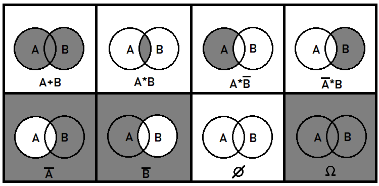
Additional algebraic operations can be composed of those presented above. For example, Boolean division is equivalent to the third and fourth situations in the above figure, since division is equivalent to multiplying by the inverse of the selected event. Strictly speaking, the first two events are enough for describing all possible events which can be composed of parts of source events. Cases with more than two overlapping events are much more difficult. In this article, we will only deal with non-overlapping events.
Market mathematics is primarily based on a concept of random walk. We will consider this concept and then it will be possible to generalize these events by the presence of patterns. Suppose we open a position with the stop loss and take profit equally spaced from the open prices. Here, we do not consider spreads, commissions and swaps. So, if we open a position for free and randomly trade in different directions and in different chart points, the profit to loss ratio will be equal to one. In other words, the number of profitable positions will be equal to the number of losing positions in endless trading. According to the above, the profit would be zero no matter how long we trade. If you apply all commissions, spreads and swaps, the final result will be negative.
The random walk may seem meaningless, as the mathematics of this process always leads to losses. But the random walk can assist in calculating the probabilities of different events. These may include closing by asymmetric stops or the average price which the chart will pass in a certain price range. We can also calculate position lifetime and other useful variables which can help in calculating risks or in your attempts to maximize profits or to minimize losses.
Probability trees and hypotheses
A very useful example for developing your frontal lobes is event trees, or probability trees. This topic originates from the Bernoulli scheme, which is the basis of all probability trees. This scheme examines the chains of non-overlapping events that follow each other. But prior to it, let us consider the total probability formula. By studying this important construction, we can proceed to the Bernoulli scheme, and them to probability trees. The formula looks like this:
- P(A) = Sum(0 ... i .... n) [ P(H[i]) * P(A|H[i]) ] - probability of event A
- P(H[i]) — probability of hypothesis H[i]
- P(A|H[i]) — probability of event A occurring within the framework of hypothesis H[i]
I'd like to say that when working with probabilities, it is better to write them in the style of hypothesis. For example, the entry P(H[k]|H[i]) would mean the following:
- The probability of event H[k] calculated relative to space H[i]
This way it is clear which event is considered space and which event is nested. The fact is that each event is a smaller event space, inside which there can be other events, which can also serve as event spaces, and so on. According to this logic, entry P(H[i]) can be written as follows:
- P(H[i]|O) — because this probability is estimated relative to O.
Now, let's split the total probability formula into parts to understand what's behind it. The formula may seem difficult at first glance, so let's make it clearer. First, I will rewrite the formula in a slightly different form:
- P(A) = (S[0] + ... + S[i] + ... + S[n]) / O = S[0]/O + ... + S[i]/O + ... + S[n]/O = (S[0]/N[0]) * ( N[0]/O ) + ... + (S[i]/N[i]) * ( N[i]/O ) + ... + (S[n]/N[n]) * ( N[n]/O )
- S[i] — the area of the specific segment of intersection of hypothesis H[i]
- N[i] — the area of the entire hypothesis H[i] (including S[i])
- O — all outcomes or the area of the entire ellipse
After small transformations, which consisted in multiplying the numerator and denominator by value N[i], we can see the probabilities that are present in the original formula:
- S[i]/N[i] ----> P(A|H[i])
- N[i]/O ----> P(H[i])
It can be visualized graphically as follows:

The outer ellipse is the event space. The central ellipse is our event, the probability of which we are looking for. Suppose it is a clock: draw the diameter of the ellipse, rotate it counterclockwise, and cut the ellipse to segments which are hypotheses. A hypothesis is only a special name for events. However, in fact they are the same events, no different from the one for which we are calculating probability.
This formula has a special case, which will assist in building the Bernoulli scheme. Imagine that the central ellipse is entirely within one of these hypotheses. Then it turns out that all the terms of this sum, which are related to the rest of the hypotheses, are automatically zeroed, because the probability of occurrence of the event A within these hypotheses is impossible or equal to zero, which eventually zeros these terms. As a result, it turns out that:
- P(A) = P(H) * P(A|H)
- H — the probability of the hypothesis, inside which the selected event is fully located.
Further, what if we assume that event A is also called a hypothesis? Why not? A hypothesis is an event, so any event is a hypothesis. Now, suppose there is another event B, which is located inside A. Then A is a hypothesis relative to B, and the previous formula is applicable to these two events:
- P(B) = P(A) * P(B|A) = P(H) * P(A|H) * P(B|A)
Insert the previous ratio instead P(A) — you can see a certain pattern in building a general formula for any number of nested hypotheses or events. What is the purpose of it? This is the direct prototype of the Bernoulli formula which we will consider a bit later. Now, there is another interesting fact to consider.
About fractals
According to the above formula, if P(A) + P(B) = 1, then this is a collectively exhaustive set of events. This means that a complete group can be composed of two arbitrary chains of hypotheses which are nested in each other. But these hypotheses can be overlapping. If we require all possible nested hypotheses be non-overlapping with the hypotheses of other chains, then automatically all chains will be non-overlapping with all chains in this event space. A graphical representation of it is quite an interesting pattern:
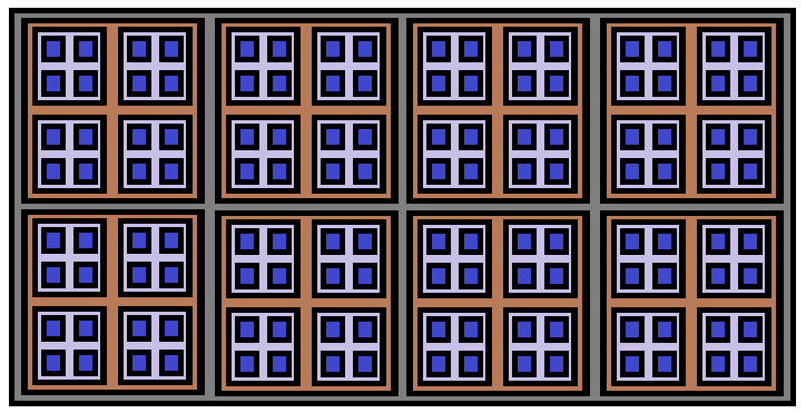
This pattern is called Fractal, because such a structure cannot be built to the end; it can be built indefinitely. In the figure above the structure is only 3 levels deep. The blue rectangles represent the end of a separate chain of probabilities. If we add up the probabilities of all these chains, they will form a collectively exhaustive set of events.
Such fractals can be well described by combinations. Combinations are based on the concept of a factorial. There is another concept, permutation, which is somewhere between factorial and combination. The permutation formula is derived from the factorial formula, and the concept of combination is derived from the permutation formula. Here are the corresponding formulas:
- n! - factorial of number n
- P(n,k) = n! / ( n - k )! — permutations from N elements by K elements
- С(n,k) = n! / ( k! * ( n - k )! ) — combinations from N elements by K elements
A factorial is the product of all natural numbers starting with 1 and ending with n, while "0! = 1". That is, the factorial of zero is equal to one. In this case it is just an exception to the rule, but I haven't seen a single case where this exception would interfere with calculations or complicate algorithms.
Permutations are a little more complicated. Imagine that you have a deck of cards, and this deck has a certain number of cards. Conduct a simple experiment: shuffle the deck and take a few carts from the deck in a completely arbitrary way, put them on the table in the order in which we they were taken out of the deck. So, permutations are the number of all possible outcomes of this experiment, while the order of the cards is also considered a unique identifier of a particular outcome. Such permutation is applicable to any desired elements.
The first card can be taken from the deck in n different ways, the second one can be taken in "n-1" ways, as the first card is no longer in the deck. And so on, till card "n-k-1". To obtain the number of all possible permutations, we need to multiply all numbers from "n-k-1" to "n". This procedure resembles a factorial. If we take "n!" and divide it by "n-k" factors, we will get the original product which is equal exactly to "(n-k)!". This is how we get the permutation formula.
The combination formula is a little more complicated, but it is also very easy to deduce. We have all possible permutations, but the order of the elements does not matter — only the cards in this set matter. Now, we need to find the number of such cases, each case having a different set of cards. In fact, each permutation already contains one of these unique sets, but we do not need all of them. Let's change the logic and try to collect all permutations of all possible combinations: it turns out that if we take a combination, no matter how we rearrange the elements in it, they will be unique. Furthermore, if we take all unique combinations and produce all possible permutations inside them, we get the following:
- P(n,k) = C(n,k) * P(k,k)
The number of all possible unique permutations inside a combination is equal to "P(k,k)", because we need to collect out of "k" variants all possible permutations for these "k" variants. By dividing both parts of the equation by "P(k,k)", we get the required combinations formula:
- C(n,k) = P(n,k)/P(k,k) = n! / ( k! * ( n - k )! )
Both permutations and combinations are widely used for various probability theory problems. When it comes to the practical applications, it is the combinations that are extremely useful to us. Combinations are used in the construction of fractal functions for a variety of purposes. Perhaps it would be more correct to call them recurrent, but for some reason I call such functions fractal (probably because they are really fractal, so it is not only a recursion but a whole tree of calls).
Bernoulli scheme
Before proceeding to studying such fractal functions, let's consider the well-known Bernoulli formula. Suppose we have a chain of identical experiments which we need to repeat several times. The experiment should result in the appearance or non-appearance of an event with a certain probability. Further, suppose we wanted to find the probability that in a chain of "n" experiments our event will appear exactly "k" times. Bernoulli formula can answer this question:
- P = C(n,k)*Pow(p,k)*Pow(q,n-k) — Bernoulli formula
- p — the probability of occurrence of the event as a result of a single experiment
- q = 1 - p — the probability that the event will not occur as a result of the experiment
Remember the formula derived earlier for probabilistic chains? Let's extend it for an arbitrary large chain length:
- P(n) = P(H[1]|O) * P(H[2]|H[1]) * P(H[3]|H[2]) * ... * P(H[k]|H[k-1]) * ... *P(H[n]|H[n-1])
- n — the number of segments in the chain
- O — the whole set of outcomes; can be denoted as H[0]
This formula calculates the probability for the exactly required chain of hypotheses to occur. The formula can be visually represented as follows:

Our formula is in the first and the largest ellipse, while another chain on the right is non-overlapping with our chain and it symbolizes some other branch from a different combination. There are exactly as many such branches as there are variants for calculating combinations in our formula. So not confuse the combinations with the combination calculation variants. The number of variants for calculating the combinations is equal to:
- n+1 (because combinations of "0" successful outcomes are also counted)
- n is the number of independent tests in the chain of experiments
Now imagine that the probabilities of all these hypotheses are equal to either "p" or "q". Then the formula is simplified:
- P(n) = Pow(p,k)*Pow(q,n-k)
- k — how many factors equal to "p" are there in the product
- n-k — how many factors equal to "q" are there in the product
It already resembles the Bernoulli formula, but it lacks the combination. If you think carefully, it becomes clear that the variants of chains with a similar probability and the quantity of "k" and "n-k" is exactly equal to "C(n,k)". Since all chains of probabilities are non-overlapping, the probability of getting one of these chains is the sum of probabilities of all such chains. Since all these probabilities are the same, we can multiply the probability of one chain by their number to get the Bernoulli formula:
- P = C(n,k)*Pow(p,k)*Pow(q,n-k)
This formula can further be expanded, for example, when we need to find the probability not of a strictly fixed combination, but of an event occurring k and more times, k and less times, and all similar combinations. In this case, it will be the sum of probabilities of all required combinations. For example, the probability of the event occurring more than k times is calculated as follows:
- P = Summ(k+1 ... i ... n)[C(n,i)*Pow(p,i)*Pow(q,n-i)]
It is important to understand that:
- P = Summ(0 ... i ... n)[C(n,i)*Pow(p,i)*Pow(q,n-i) ] = 1
in other words, all possible chains form a collectively exhaustive event set. Another important equation is:
- Summ(0 ... i ... n)[C(n,i)] = Pow(2,n)
It is logical, given that each segment of the probability chain has only two states: "the event occurred" and "the event didn't occur". The state when the event didn't occur is also an event which implies that another event happened.
Combinations have another interesting property:
- C(n,k) = C(n,n-k)
It is derived as follows: calculate "C(n,n-k)" and compare with "C(n,k)". After some minor transformations, we can see that both expressions are identical. I have created a small program based on MathCad 15 in order to check all of the above statements:
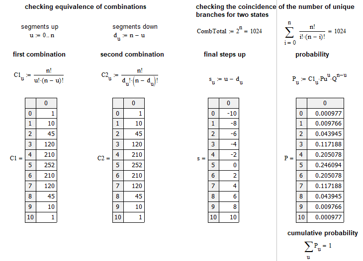
This example is close to the market. It calculates the probability that out of n steps the market will move u steps up. A step is the price movement at a certain number of points up or down, relative to the previous step. The graphical array of probabilities for each "u" can be shown as follows:
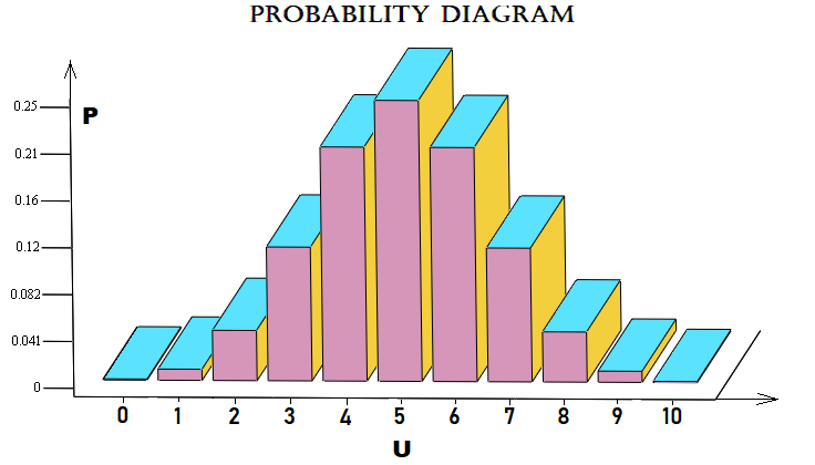
For simplicity, I used a Bernoulli scheme with 10 steps. The file is attached below, so you can test it. You do not necessarily need to apply this scheme to pricing. It can also be applied to orders or anything else.
Creating the first fractal
Special attention should be paid to the problems related to stop loss and take profit levels. We should somehow calculate the probability of a deal to be closed by stop loss or take profit when we know the values of stop loss and take profit in points (distance from the current price). This value can be calculated at any point, even if this is no longer the open price, as all these aspects are directly dependent on the pricing mechanisms. In this example, I want to demonstrate the proof of the formula using fractals. In case of a random walk, this probability can be calculated as follows:
- P(TP) = SL / ( TP + SL ) - the probability of hitting take profit
- P(SL) = TP / ( TP + SL ) - the probability of hitting stop loss
- SL — point distance to stop loss
- TP — point distance to take profit
These two probabilities form a collectively exhaustive event set:
- P(TP) + P(SL) = 1
According to this formula, for random trading, the math expectation of such strategies will be zero, if we exclude spread, commission and swap:
- M = P(TP) * TP - P(SL) * SL = 0
This is the simplest case when we set a fixed stop level. But it is possible to generalize it to absolutely any strategy. Now, let's prove the formula using the same MathCad 15. I have been working with this program for a long time. It can produce calculations of almost any complexity level, even using programming. In this example, in addition to proving the above formulas, we will see the first example of constructing a fractal formula. Let's start by sketching the price movement process. We cannot use continuous functions here, but only discrete ones. For this, let's take our conditional order and calculate stop level distances up and downward, after which let's split these segments into parts with equal steps, so that each step includes an integer number of steps. Imagine that the price moves by these steps. Since the steps are equal, the probability of a step in any of the two directions is 0.5. We need a graphical representation to implement the appropriate fractal:
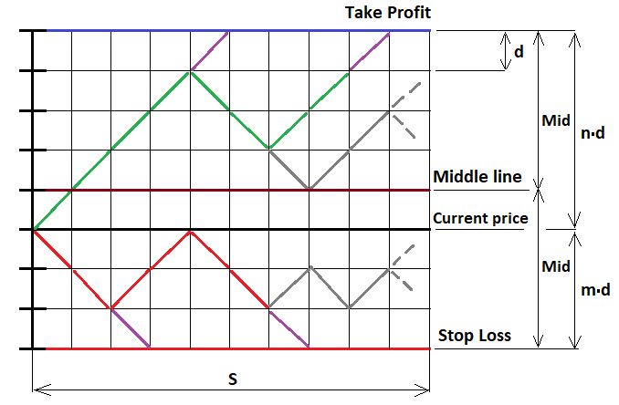
To solve this problem, let's consider three possible fractal continuation cases:
- We are above the middle line ( U > MiddleLine )
- We are below the middle line ( U < MiddleLine )
- We are at the middle line level ( U = MiddleLine )
"U" is the total number of steps "u-d" up relative to the open price. If the point from which we are going to continue building the fractal is below the price, then U takes negative values in accordance with the function. If we are at the middle line, the number of steps that we can take without fear of crossing the line is one less than Mid. But before proceeding with the construction, we must limit the fractal construction to the number of steps that the price or orders can make. If the number of steps exceeds the required number, we must interrupt its further construction. Otherwise, we will get an infinite recursion, from which it will be impossible to exit. Its computation time will be equal to infinity.
In the figure, I drew several purple steps — at these points we collect the probabilities and sum them into a common variable. After that we need to turn our chain up or down, depending on which border the chain touched, so that it can continue moving further to build new nested fractal levels. In other points, we can freely build full fractal levels based on Bernoulli scheme.
When it is possible to create a tree based on Bernoulli scheme, we must first determine the number of steps which we can make, taking into account extreme cases, when all steps are only up or only down. For all the three cases the value is equal to:
- (n - 1) - U — when our chain is already above the middle line (since an increase in U causes a decrease in the distance to the upper boundary)
- (m - 1) + U — when our chain is already below the middle line (since a decrease in U causes a decrease in the distance to the lower boundary)
- (floor(Mid)-1) — when our chain is exactly at the middle line
- n — the number of upper segments
- m — the number of lower segments
- floor — the function discards the fractional part (this might not be necessary)
First we need to calculate two auxiliary values:
- Mid = (m+n)/2 — half of the range width (in steps)
- Middle = (m+n)/2 - m — the "U" value for the middle line (in steps)
These values will later be used to describe the fractal branching logic. As for now, we will create the fractal only for the cases where "n>=m". However, this data is not enough to build a fractal. In order to be able to build deeper fractal levels, it is necessary to redefine "U" for each new combination from the Bernoulli scheme and to pass it to a new fractal level. In addition, it is necessary to correctly increment the number of steps performed and also to correctly pass them further. Similarly, we need to collect the probability of the entire chain using the multipliers of the next fractal level and to pass the probability of the intermediate chain further, to the next level, until this process ends with a successful crossing of the required border. The below image explains these three variants:

According to this diagram, we can now write what the values "NewU" and other auxiliary values will be equal to for each presented case. Let's consider an example of constructing a fractal to calculate the probability of crossing the upper boundary:
For case 1:
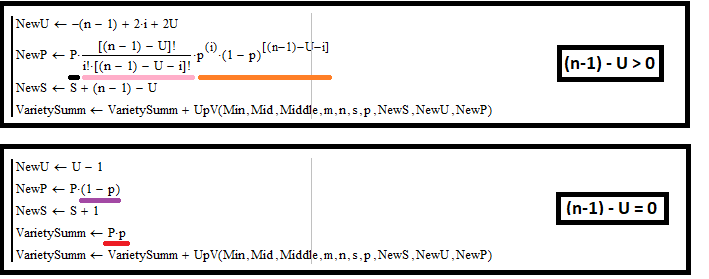
Let's take a look at the upper picture and describe mathematically what is happening there. This figure shows an abstract from my program in MathCad 15. The whole code of the program is attached below. Here I provide the most important details which are the basis of the fractal. The first rectangle is in a loop, and it iterates by "i" to describe all possible combinations. This logic can be repeated in the MetaEditor IDE. Let's start with the first illustration in the diagram. To define "NewU", we first need to define some fundamental formulas:
- ( n - 1 ) - U = f — it is the number of steps of the future combinations tree (the distance is determined by the distance to the nearest border of the fractal range)
- u + d = f — the same value, but expressed in terms of the number of rising and falling segments
- s = u - d — the number of final steps, expressed in terms of falling and rising segments
- u = i — this is because my program uses iteration by "i" (should be remembered)
In order to calculate all the required values, we need to express "s" through "U" and "i". For this, we need to exclude variable "d". First express it, and then substitute it into the expression for "s":
- d = f - u = f - i = ( n - 1 ) - U - i
- s = i -( n - 1 ) + U + i = -( n - 1 ) + 2*i + U
Next, using the found "s", find "NewU" and all values to be passed to the next fractal level:
- NewU = s + U = -( n - 1 ) + 2*i + 2*U - our new "U" to be passed to the next fractal level
- NewP = P * C(f,i) * Pow(p,i) * Pow(1-p,f-i) = P * C( ( n - 1 ) - U ,i) * Pow(p,i) * Pow(1-p,( n - 1 ) - U -i) — our new probability of chain "P" to be passed to the next fractal level (obtained by multiplying by the probability of the new segment of the chain)
- NewS = S + f = S + ( n - 1 ) - U — new "S" to be passed to the next fractal level
Now, take a look at the lower rectangle. Here we handle cases when the step chain has reached the upper border of the range. Two cases should be handled here:
- Collecting the probability of the chain that intersects with the border (underlined in red)
- Similar actions, incrementing new values which we will pass to the next fractal level
This case is very simple as there are only two possible variants:
- Touching the border
- Reverting from the border
These actions do not need the Bernoulli scheme, as each case implies only one step. The probability of the reversal is additionally multiplied by "(1-p)", because the probability of intersection is "p", and these two events should form a collectively exhaustive set, as is clear from the previous calculations. Steps are incremented by 1, and "U" is decreased by "1", because this is a reflection which goes down. Now we have everything to correctly build this case. These rules will be identical for building the main fractals, which we need for completely different cases.
For case 2:
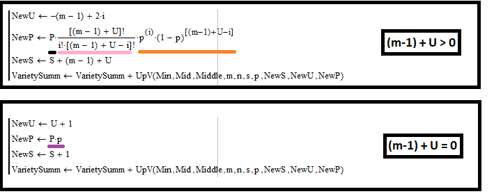
Calculation is almost similar for this case. The only difference is that "f" takes a different value:
- ( m - 1 ) + U = f
Again, express "s" through "U" and "i", using the same formulas from the previous case:
- d = f - u = f - i = ( m - 1 ) + U - i
- s = i -( m - 1 ) - U + i = -( m - 1 ) + 2*i - U
Similarly, find all other values that we need to pass to the next fractal level:
- NewU = s + U = -( m - 1 ) + 2*i - out new "U" to be passed to the next fractal level
- NewP = P * C(f,i) * Pow(p,i) * Pow(1-p,f-i) = P * C( ( m - 1 ) + U ,i) * Pow(p,i) * Pow(1-p,( m - 1 ) + U -i) — our new probability for chain "P" to be passed to the next fractal level
- NewS = S + f = S + ( m - 1 ) + U — our new "S" to be passed to the next fractal level
The lower rectangle is almost identical to the previous case, except that we increase "U" by 1, because the reflection goes up and so "U" is increased. Probabilities are not collected in this case, because we are not interested in the intersection with the lower border in this fractal. Now, here is the last case, when the chain occurred at the middle line of the range.
For case 3:

Define "f":
- floor(Mid) - 1 = f
Find "s":
- d = f - i = floor(Mid) - 1 - i
- s = i - d = -(floor(Mid) - 1) + 2*i
Finally, find the values to be passed to the next fractal level:
- NewU = s + U = -(floor(Mid) - 1) + 2*i + U
- NewP = P * C(f,i) * Pow(p,i) * Pow(1-p,f-i) = P * C( floor(Mid) - 1 ,i) * Pow(p,i) * Pow(1-p,floor(Mid) - 1 - i) — our new chain probability "P" to be passed to the next fractal level
- NewS = S + f = S + (floor(Mid) - 1) — our new "S" to be passed to the next fractal level
A distinctive feature of this case is that the block does not collect probabilities, because probabilities can only be collected at the border values of "U", where probability chains are also reflected back into the chain so that they can spread further. Creation of a fractal for calculating the probability of crossing the upper border will be identical, but the probabilities will be counted in the second case, not in the first one.
An interesting feature in the construction if such fractals is the mandatory presence of the Bernoulli formula in such functions. The combinations are highlighted in pink, and the products of probabilities are shown in yellow. These two multipliers together form the Bernoulli formula.
Now, let's check two things at the same time: the correctness of construction of the entire fractal and the assumption that the expected payoff only depends on the predictive ability. The steps can be presented as points and as deals. In the latter case the points should be multiplied by the appropriate proportionality coefficient, which depends on lots and tick size. Here we will use points - this representation is universal:
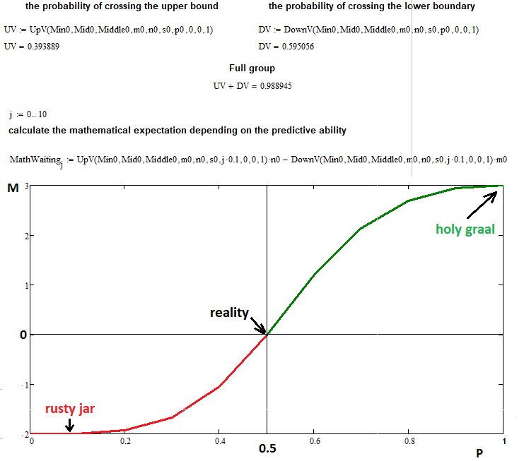
In this example, I used the following input data to plot the mathematical expectation versus the probability of a step up:
- n = 3 — number of upper segments
- m = 2 — number of lower segments
- s = 22 — number of allowable steps for a chain reaction of the fractal function (if you increase this value, it will create extra load on the computer, so this number of steps is quite enough)
- 0 ... 0.1 ... 0.2 ...... 1.0 — dividing the range of up step probabilities into 10 parts with a step of 0.1
As you can see, for the probability of 0.5 the mathematical expectation for our deals is equal to zero, as previously predicted by the formula. At extreme points 0 and 1, the function value tends to "n" and "-m", which confirms our assumptions. The fractal has successfully completed its task, although it revealed a drawback: a great increase in the computation time and complexity. However, it is quite acceptable to wait for a couple of hours or even a day for similar tasks.
This fractal only works for cases when n >= m, i.e. when the distance till the upper border is greater than the distance till the lower border, but there is no need to provide this in the fractal. This construction can be mirrored: if n < m, we can calculate the fractal by passing m instead of n and n instead of m to it. Then switch the probabilities and obtain the desired result. Such fractals can be used not only to prove formulas, but also for a reverse process. Some formulas can only be obtained as a result of using fractals.
Summary
I think the following very important conclusions have been made in this article:
- Probability theory combined with programming can provide a theoretical basis for describing many of the market processes.
- Fractals combined with the main provisions of probability theory can answer the most difficult questions.
- We have seen an example of creating a rather complex fractal.
- The whole theory was tested in practice using programming in the MathCad 15 environment.
- The article has proved that the Bernoulli scheme provide opportunities for creating any fractals with two step states.
Conclusion
I hope the reader could see something new in this material, which can be used in practice for trading. While working on this article, I tried to convey the full power of discrete mathematics and probability theory, in order to prepare you for another difficult task — describing market processes using fractal-probability chains. I tried to combine all the main provisions of probability theory into one material, which can further help in solving complex task for practical trading. Also, I tried to remove all irrelevant details. The next article will provide new examples of practical application of fractals and answers to other important questions.