Developing a self-adapting algorithm (Part I): Finding a basic pattern

Maxim Romanov | 8 February, 2021

Introduction

Any trading algorithm is generally a tool which may bring profit to an experienced trader or instantly destroy a deposit of an inexperienced one. The issue of creating a profitable and reliable algorithm is that we cannot understand what needs to be done in order to earn money and what methods are used by "successful traders". While HFT, arbitrage, option strategies and calendar spread-based systems boast a solid theoretical basis clearly stating what needs to be done to make profit, the algorithms based on price analysis and fundamental data are much more ambiguous. This area has no full-fledged theoretical basis that would describe pricing making it extremely difficult to create a stable trading algorithm. Trading turns into art here, while science helps systematizing everything.

But is it possible to create a fully automated trading algorithm based only on the analysis of price changes working on any trading instrument without optimization and with no need to manually adjust parameters for each trading instrument separately? Is there an algorithm you can simply apply to a necessary trading instrument chart so that it immediately defines profitable parameters for it? 

Is it possible for an algorithm not to lose regardless of market changes? I believe, it is possible, albeit difficult to achieve. There are two ways to solve this issue:

1. Use neural networks with machine learning and get a "black box" analyzing the market and making profit following its own criteria. Despite the apparent obviousness and attractiveness of this approach, it has its own complexities. If it were so easy to do, then such companies as Google and Yandex, with their vast experience in using machine learning and large budgets, would have solved this problem long ago, or at least they would have been among the leaders in the analysis of market data and the quality of forecasts. I believe, it is possible to create such an algorithm. It should be constantly refined as technology develops in order to remain competitive. After all, you will have to compete with tech giants.
2. Study the pricing patterns, develop a theoretical model of price formation and create an algorithm creating as much factors affecting pricing as possible. In my opinion, this method is even more complicated than machine learning, but I think it is real as well. Such an algorithm will improve along with the development of the theoretical background and developer's knowledge. It will also require constant modernization.

I decided to use the second method, namely create a full-fledged theory and develop an algorithm based on it. I am going to develop the algorithm in a series of articles moving from a small pattern to a large project. Besides, I will show how to find and study patterns while improving work efficiency.

The first algorithm will be developed only for FOREX and MetaTrader 4 terminal. Along the way, it is to evolve into a universal MetaTrader 5 algorithm working both in FOREX and exchanges.

Basic pattern

Let's start from searching for the basic pattern that will form the basis of the algorithm. This pattern should be fundamental and inherent in most markets in order to easily scale it to any market in the future. The scalability for any market suggests that the algorithm is truly self-adapting.

To begin with, let's try to define why it is difficult to earn consistently in the market. It is all about direct competition. The task of some traders is to conclude a profitable deal with others, but the problem is that each of the parties wants to conclude a profitable deal and someone definitely gets a loss. Therefore, the market should not have stable simple patterns that everyone can notice.

In my first article "Price series discretization, random component and "noises", I wrote about a random component in the market and the fact that the distribution of increments for a price series is very similar to the distribution of increments for a random walk. At the first glance, the price series seems to have no patterns, everything happens randomly and it is impossible to make stable money on this.

Therefore, as a basic rule, I took that there are exactly the same number of rising candles for any instrument as there are falling ones. This is a very simple pattern, and any deviation from it leads to stable earnings for everyone noticing it. I think, many will notice it since it is so simple. But as we know, it is impossible for everyone to make money, so there can be no significant alteration of the number of falling candles from the number of growing ones in the long term. This is implicitly stated in the mentioned article. Theoretically, there can be deviations from this rule, because I did not check all the tools, but only about a hundred of them. However, it is not so important at this stage. 

For example, let's take 100,000 GBPUSD H1 candles for any period and calculate how many of them are rising and how many are falling. I took the period of 100,000 candles from 2020.10.27 to the past. The period contains 50,007 bullish and 48,633 bearish candles. For the remaining candles, the opening price is equal to the closing one. In other words, GBPUSD features 50.7% bullish and 49.3% bearish candles, the remaining candles have Open = Close. The values are roughly equal. If we take a larger sample, the result will tend to 50%.

I will not measure every instrument within this article. I observed hundreds of instruments and the results were similar everywhere. But to be convincing, let's take an instrument from a completely different market GAZP (Gazprom) M15 and measure the number of falling and growing candles on 99,914 candles. The result is 48,237 bullish and 48,831 bearish ones. The remaining ones are neutral. As you can see, the number of bearish and bullish candles is approximately equal.

This pattern is not only present on a large number of instruments, but also remains on any timeframe. To make sure of this, let's analyze GBPUSD M1 and take the steadily growing AAPL stock on M15. I combined all the data into a table.

Symbol	Timeframe	Total candles	Total bullish candles	Total bearish candles
GBPUSD	M1	100,000	50.25%	49.74%
GBPUSD	H1	100,125	50.69%	49.30%
GAZP	M15	99,914	49.69%	50.30%
AAPL	M15	57,645	50.60%	49.40%

According to the table, the ratio of rising to falling candlesticks tends to 50% on the considered instruments and is valid for all considered timeframes. The XLSX file containing data used in my measurements, as well as the results, is attached below.

The results shown in the table confirm the conclusion that the statistical parameters of the price series over a large number of samples are very similar to the random walk parameters. Moreover, on a small number of samples, there will be deviations from the reference distribution. The algorithm will be based on the assumption that the distribution of the increments for the price series is only superficially similar to normal.

On a small number of samples, the distribution shape differs from the reference one, while with an increase in the number of samples, the shape tends to the reference one. Most importantly, the speed, with which the distribution tends to the reference one, is individual for each instrument and is quite stable. 

Figure 1

Figure 1 visualizes all that has been described above. The reference distribution of increments is shown in red, while the distribution of increments for a price series with a large number of samples is shown in black. The distribution of price series increments on a small number of samples is shown in violet, green and blue.

The fundamental regularity inherent in a large number of trading instruments has been found and an assumption where to look for a profit has been made. The number of bearish candles = the number of bullish ones, and when a deviation from the equilibrium occurs, the rate of return to the equilibrium for each instrument is individual, stable and fluctuates within certain limits. I will use this pattern to make a profit.

Developing a test algorithm

Maximum number of positions in a series

During trading, a position is filled with a series of orders, so we need to limit the maximum number of positions. To do this, we need to calculate the number of candles, at which the excess can be straightened up to 50%. We use the sample that triggered the start of the series (consisting of N candles), calculate the number of dominant candles, subtract the remaining candles from it, add it to the number of candles in the initial sample and multiply by the К adjusting factor. The К ratio is indirectly linked to the statistical characteristics of the instrument.

This is how we obtain the expected number of candles, at which the deviation from 50% should disappear.

R=(N+NB-NM)*K
N - number of candles in the sample featuring an excess above the threshold
NB - number of dominant candles
NM - number of remaining candles
K - adjusting factor defined in the settings

Next, we need to calculate the maximum number of positions the robot is to open. To achieve this, we need to subtract the number of candles in the initial N sample from the total number of candles R. The result is the maximum number of positions E the robot should not exceed in the series.

E=R-N
Е - maximum number of positions in the series
R - total number of candles, at which the return to 50% is planned

This algorithm is not self-adapting yet, but the first steps are taken and the number of positions is adjusted from the number of candles in the initial sample.

Lot selection

The algorithm has been created to check the pattern. Therefore, we need to add several settings to determine the lot. Suppose that the lot size depends on the expected number of positions in the series. The more positions in the series, the smaller the lot. To do this, add two settings: Depo and RiskPerc. For simplicity, let's assume that $1000 = lot ($500=0.5 lot). Take the value from the Depo setting and multiply it by RiskPerc. Divide the obtained value by the maximum number of positions E and round it to the nearest correct value. This is how we get the lot size of one position.

We need to add the lot auto increase function if the deposit grows. In that case, if Depo = 0, the current deposit value is multiplied by RiskPerc and the lot for opening positions is found using the obtained value.

Closing positions

Closure occurs in several cases:

1) The total profit on open positions reaches the values set in CloseProfit. Since the number of positions opened by the EA is not constant and the lot size may change, it would be incorrect to set the fixed profit in USD. We need the USD profit depend on the current number of open positions and the total lot in the market. To do this, we need a concept of "profit per lot".

The CloseProfit setting sets the profit for the total position of 1 lot, and the robot re-calculates the profit for the number of lots it opened. If we have 10 open positions at 0.01 lot each, the total lot is 0.1. So, in order to get the profit value for closing a position, Profit = CloseProfit * 0.1. Adjust the profit to close positions each time the number of positions changes. As a result, when the total profit becomes greater than or equal to the calculated Profit value, the EA closes positions.

2) When the current excess percentage becomes less than or equal to ClosePerc. ClosePerc sets the excess percentage of prevailing candles to generate a signal for closing the series of positions. When the first position was opened, the excess was found on the N number of candles. Now, with each new candle, the number of candles increases becoming N+1; N+2; N+3 etc... With each new candle, we need to check the current excess percentage of prevailing blocks on a sample with the number of candles increasing by 1. Complete the series after the condition is met.

3) Upon reaching MinEquity. If the current funds have fallen below the set value, you need to complete the open series and avoid opening new ones until the funds increase. This is the Stop loss function protecting the deposit from losses.

Test

The algorithm is quite primitive. It is unable to adapt to changing market conditions and is used only to check the idea viability. Therefore, I will select the settings using optimization. The optimization is to be performed by enumerating all options with no genetic algorithm. The EA was developed back in 2014 and made for MetaTrader 4. I will first test it on GBPUSD H1. I will set the artificially high spread of 40, so that the optimization is performed in non-perfect conditions to ensure a certain margin of stability in the future. An increased spread is needed because the EA controls the current profit on open positions and is influenced by the spread.

I will optimize only three conditions: the minimum number of candles MinBars, percentage for opening positions OpenPerc and profit per lot CloseProfit. Presumably, the larger the minimum number of candles for analysis and the higher the opening percentage, the more reliable, but less frequent, the signals will be. CloseProfit indirectly depends on volatility. Therefore, before optimization, you need to look at the volatility of the instrument and set an adequate range. The optimization is to be performed for the year from 2019.11.25 to 2020.11.25 on H1.

Figure 2. Optimization results

The brute force optimization is necessary to see how the parameters affect the result and how the results converge with the assumptions about how the algorithm should work in theory. Figure 2 shows some of the results. We need to enable sorting by maximum profit and select the settings having the most adequate indicators of drawdown and profitability. The highlighted settings seem to be fine.

The further analysis of the optimization results shows that an increase in MinBars and OpenPercent reduces profitability and drawdown. Next, I took the highlighted parameters, tested them within a year, obtained results and defined what changes if MinBars and OpenPercent are increased/decreased. My conclusion is that the number of deals decreases and the signal reliability increases along with an increase of MinBars and OpenPercent. This means, we need to find the balance between profitability and drawdown.

For trading, I took deliberately more conservative parameters to ensure a margin of safety for changing market conditions. Figure 3 below shows how the EA opens positions.

Figure 3. Opening positions

Figure 3 shows that a position is made of several deals if necessary. The entry signal is stretched over time. The first version of the algorithm features a rough signal considerably stretched in time at some points. It looks more like a fuzzy input rather than a standard averaging. This is an area with fuzzy boundaries, in which bearish candles are more likely than bullish ones. It is possible to make profit from this probability.

The algorithm remains reliable at MinBars = 70, but I set it to 80 so that there is a margin for fluctuations in the trading instrument characteristics. The logic is similar when selecting the CloseProfit parameter. In the example, it is equal to 150. In case of a lesser value, the algorithm becomes more stable but the profit is reduced. If increased up to 168, the algorithm is no longer reliable, therefore I will stick to 150. As a result, we have obtained the profitability graph for a year as in Figure 4. CloseProfit is nothing more than the average volatility converted into USD.

Figure 4. GBPUSD H1, 2019.11.25 - 2020.11.25

The deposit is set to $10,000 for optimization. After completing the research, we can set the sum back to the optimal one. The test and optimization were performed in the reference point mode because the algorithm works on close prices, so the events within a candle are of no importance to it. Figure 5 shows the test for the same period in the "Every tick" mode.

Figure 5. GBPUSD H1, 2019.11.25 - 2020.11.25 "Every tick" mode

According to Figure 5, the profit has even slightly increased in the "Every tick" mode because the test has become more accurate. The profitability graph remains almost completely the same. Both tests have yielded an excellent profit factor of just over five.

It would be wrong to draw conclusions about the pattern reliability based on tests for one optimized year, so let's see how many years the algorithm is able to last with these parameters in the past. Figure 6 shows the test result outside the optimized period.

Figure 6. GBPUSD H1, 2001.01.01 - 2020.11.25

Figure 6 shows the backtest since 2001 with the same parameters that were obtained during the one-year optimization from 2019.11.25 to 2020.11.25. The test shows that the drawdown has increased by only a couple of dollars on such a large interval, while the profit increased significantly and the profit factor rose to 7.5. The test was carried out for the deposit of $3000 with no refinancing in order to understand how the pattern behaves over long periods of time. 

The fact that the optimization has been carried out in a year, while the algorithm shows a stable result for 20 years, indicates that the pattern is quite stable and the parameters are not adjusted to the history. For some reason, the GBPUSD pair does not deviate greatly from its inherent statistical characteristics. 

It would be wrong to draw conclusions based on the test of a single currency pair and timeframe. Therefore, let's consider the tests for EURUSD. As in the previous case, the optimization was carried out in a year from 2019.11.25 to 2020.11.25 on H1. I approached the choice of parameters in the same way as in the previous case. The results are shown in Figure 7.

Figure 7. EURUSD H1, 2019.11.25 - 2020.11.25

As we can see in Figure 7, the profitability on EURUSD is lower than on GBPUSD, while the drawdown is slightly larger. The profitability graph shows that there was a segment with multiple opened positions. After slightly tightening the MinBars and OpenPercent parameters, we are able to reduce the number of positions and, consequently, drawdown. Let's move on to the long-period test. Figure 8 displays testing EURUSD from 2007.01.01 to 2020.11.25.

Figure 8. EURUSD H1, 2007.01.01 - 2020.11.25

Trading EURUSD is not so stable compared to GBPUSD. The period of stable work using the data that is further back in time has turned out to be six years less. The result is still good. Optimization of parameters was carried out in a year, and stable work lasted almost 14 years. This fact again suggests that the parameters were not simply adjusted to the history, and the trading instrument features a fairly stable pattern.

Next, you need to check how the algorithm behaves on other timeframes. Theoretically, with a decrease in the timeframe, stability should decrease, because the size of candles on a lower timeframe decreases significantly relative to the spread. Consequently, there will be less profit and more trading costs. Besides, on smaller timeframes, the entry point may become even more stretched in time leading to more open positions and, accordingly, greater drawdowns.

Let's conduct a test on GBPUSD M15. Like in the previous case, the optimization is to be performed for the year from 2019.11.25 to 2020.11.25. But I will not display the optimization graph for a year. Instead, I will display the largest possible interval the algorithm is able to pass smoothly.

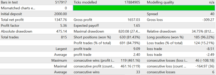
Figure 9. GBPUSD m15 2000.01.01-2020.11.25

Figure 9 shows the test of GBPUSD M15 conducted from the year of 2000. But the number of entry signals and positions is small. As I wrote above, the lower timeframe demonstrates less stability, and the settings turn out to be very conservative. The entry signal is rarely generated, the profitability is not high, but is adequate relative to the drawdown.

Next, let's conduct the test on the higher timeframe GBPUSD H4. H4 has few candles for optimization. Therefore, I will perform optimization on a two-year segment from 2018.11.25 to 2020.11.25. The result will be shown on the maximum interval.

Figure 10. GBPUSD H4 2000.01.01-2020.11.25

H4 shows a stable result within almost 20 years from 2000.01.01 to 2020.11.25. Like in the previous cases, the entire optimization boils down to finding the balance between profit and reliability. The conservative settings from M15 work reliably on both H1 and H4. But there is no point in them there due to very rare signals and a small number of deals.

You can also test any other trading instrument. Depending on a symbol, the algorithm works better or worse. But the trend continues — one-year optimization allows for a stable work for several years. Below are the results for GBPJPY H1. Optimization was carried out for a year, the result is shown in Figure 11.

Figure 11. GBPJPY 2009.01.01 - 2020.11.25

GBPJPY shows a stable backtest since 2009. The result is not as impressive as in the case of GBPUSD, but it works. 

The EA features the ability to re-invest the earned funds. You need to use it. Until now, I showed the tests with conservative settings. But what if we set very aggressive settings and enable a lot increase? I am not a fan of high risks, but let's see what the algorithm is capable of. I will perform the test on GBPUSD from 2006.01.01 to 2020.11.25 in the "Every tick" mode. Of course, it is possible to test another symbol. The spread is reduced to 20. This is slightly above average. Figure 12 shows the backtest result for almost 15 years.

Figure 12. GBPUSD from 2006.01.01 to 2020.11.25, aggressive settings

As you may remember, the algorithm uses close prices. Therefore, this result is not a "test grail". In addition, the adequate spread of 20 is set. The algorithm's trading result on the real market usually coincides with the one obtained in the tester. I have never used it to trade with such aggressive settings. Besides, it is impossible to take into account real spreads in MetaTrader 4, so I will not argue that it would have passed this period as well in real trading.

Analyzing the results

The EA is simple and easy to optimize. Optimization for a short period of time and the use of non-optimal parameters in advance allow it to remain stable for several years, and sometimes dozens of years. This suggests that the found pattern is not accidental and is really present on the market. However, the algorithm is quite "rigid" as it has few degrees of freedom and operates with rigidly specified parameters. If a price series goes beyond the capabilities of the algorithm, then it immediately loses its stability. 

Most importantly, it can be used on any timeframe starting with the one having the candle size considerably exceeding the spread and commission. As the timeframe increases, the stability grows up to the daily timeframe. However, the requirements for the deposit also increase since the candle size becomes significant causing large drawdowns.

We can conclude that the price series is only superficially similar to a random walk as I described in my first article "Price series discretization, random component and noise". The price series contains at least one hidden pattern.

On the other hand, I know and thoroughly understand the pattern that allows making profit, which means it is time for some serious modernization.

Usage in trading

The big drawback of the current algorithm is its low return relative to risks. We need to be honest with ourselves and understand that there are risks (just like anywhere else). But while the development of improvements is in progress, we may use the EA for trading. To do this, we need to raise its profitability and maintain the drawdown level. It is necessary to use the algorithm features. It rarely generates signals for trading instruments and, as a rule, they are significantly spaced in time for different trading instruments. Most of the time there is no trading on the instrument. We need to fill these "downtime". 

Generally, there is no stable correlation of signals for different instruments. We should use this feature to increase profit while maintaining the drawdown level.

To increase profitability, we need to analyze several instruments simultaneously. When a signal appears for one of the instruments, open positions on it. If positions are opened for one instrument, ignore the series start signals from other symbols. This allows using time as efficiently as possible, increase the number of signals, and, accordingly, raise profit proportionally. The maximum drawdown remains at one instrument level.

Series start signals are weakly correlated not only between independent symbols but also between different timeframes of the same symbol. Therefore, it is possible to use time even more efficiently and achieve a situation where there are almost always open positions in the market by using three timeframes of the same symbol in trading. The drawdown level remains at the same level, while the profit grows significantly.

Several modifications were made for working on real accounts:

1) Add nine new independent trading instruments, each with its own parameters. This allows the algorithm analyze and trade 10 trading instruments at once. It is possible to optimize parameters for any instrument to one degree or another, so the decision seems logical.

2) Limited simultaneous opening of positions for several trading instruments. The MaxSeries parameter is added for that. If set to 1, trading is performed only on one instrument. If 2, positions can be opened simultaneously on two instruments, and so on. This will make it possible for the EA to generate position open signals more often, using its "free time". The profit is increased proportionally, while the maximum drawdown remains at the level of one instrument.

MetaTrader 4 tester is unable to perform multi-currency tests. But if more than one symbol is traded, the drawdown probably increases proportionally to the square root of the number of simultaneously traded instruments, provided that there is no correlation between signals of different instruments. If we expect a drawdown of $1000, then, trading three instruments simultaneously, we can expect an increase in the drawdown to the level of $1000*root(3)=$1732.

3) Added limitation on the minimum number of "MinEquity" funds. Upon reaching this value, trading stops and positions are closed. This is necessary in order to plan the risks and adhere to them.

4) The EA can be used on several timeframes simultaneously to increase profitability. According to my tests, position open signals usually have a correlation between different timeframes, although it is far from 100%.

I used the EA to trade on 25 currency pairs, as well as on H1 and H4 timeframes simultaneously with conservative settings and managed to maintain the profitability at 10% per month. On another account, with slightly more aggressive settings, I managed to achieve a profitability of 15% per month. There were a lot of deals.

Conclusions and further development

• A non-conventional trading method has been found;

• The selected basic pattern has turned out to be universal and is present on tested trading instruments;

• The pattern is simple and clear. We need to study the reasons for its occurrence and develop ways to improve the signal quality;

• The algorithm is perfectly optimized and remains stable for a long time;

• The entry point is strongly stretched in time. We need to work on better localization of the position open signal;

• Unaccounted factors lead to a loss of the algorithm stability over time;

• It is necessary to continue the development of the theoretical model to reduce the number of unaccounted factors with each new version and, as a result, take into account all possible factors influencing the pattern;

• The next version of the algorithm should become more flexible and should already begin to slightly adjust its parameters for market changes.

The next article is to be devoted to mechanisms I have developed to improve the algorithm reliability and flexibility.

The EA code and the appropriate requirements specification are attached below.

The author of the idea and requirements specification is Maxim Romanov. The code has been written by Vyacheslav Ivanov.