Neural networks made easy (Part 6): Experimenting with the neural network learning rate

Dmitriy Gizlyk | 8 January, 2021

Introduction

In earlier articles, we considered the principles of operation and methods of implementing a fully connected perceptron, convolutional and recurrent networks. We used gradient descent to train all networks. According to this method, we determine the network prediction error at each step and adjust the weights in an effort to decrease the error. However, we do not completely eliminate the error at each step, but only adjust weights to reduce the error. Thus, we are trying to find such weights that will closely repeat the training set along its entire length. The learning rate is responsible for the error minimizing speed at each step.

1. The problem

What is the problem with learning rate selection? Let us outline the basic questions related to the selection of the learning rate.

1. Why cannot we use the rate equal to "1" (or a close value) and immediately compensate the error?
In this case, we would have a neural network overtrained for the last situation. As a result, further decision will be made based only on the latest data while ignoring the history.

2. What is the problem with a knowingly small rate, which would allow the averaging of values over the entire sample?
The first problem with this approach is the training period of the neural network. If the steps are too small, a large number of such steps will be needed. This requires time and resources.

The second problem with this approach is that the path to the goal is not always smooth. It may have valleys and hills. If we move in too small steps, we can get stuck in one of such values, mistakenly determining it as a global minimum. In this case we will never reach the goal. This can be partially solved by using a momentum in the weight update formula, but still the problem exists.

3. What is the problem with a knowingly large rate, which would allow the averaging of values over a certain distance and avoid local minima?
An attempt to solve the local minimum problem by increasing the learning rate leads to another problem: the use of a large learning rate often does not allow minimizing the error, because with the next update of the weights their change will be greater than the required one, and as a result we will jump over the global minimum. If we return to this further again, the situation will be similar. As a result, we will oscillate in around the global minimum.

These are well known problems, and they are often discussed, but I haven't found any clear recommendations regarding the learning rate selection. Everyone suggests the empirical selection of the rate for each specific task. Some other authors suggest the gradual reduction of rate during the learning process, in order to minimize risk 3 described above.

In this article, I propose to conduct some experiments training one neural network with different learning rates and to see the effect of this parameter on the neural network training as a whole.

2. Experiment 1

For convenience, let us make the eta variable from the CNeuronBaseOCL class a global variable.

double   eta=0.01;
#include "NeuroNet.mqh"

and

class CNeuronBaseOCL    :  public CObject
  {
protected:
   ........
   ........
//---
   //const double      eta;

Now, create three copies of the Expert Advisor with different learning rate parameters (0,1; 0,01; 0,001). Also, create the fourth EA, in which the initial learning rate is set to 0.01 and it will be reduced by 10 times every 10 epochs. To do this, add the following code to the training loop in the Train function.

         if(discount>0)
            discount--;
         else
           {
            eta*=0.1;
            discount=10;
           }

All the four EAs were simultaneously launched in one terminal. In this experiment, I used parameters from earlier EA tests: symbol EURUSD, timeframe H1, data of 20 consecutive candlesticks are fed into the network, and training is performed using the history for the last two years. The training sample was about 12.4 thousand bars.

All EAs were initialized with random weights ranging from -1 to 1, excluding zero values.

Unfortunately, the EA with the learning rate equal to 0.1 showed an error close to 1, and therefore it is not shown in charts. The learning dynamics of other EAs is shown in the charts below.

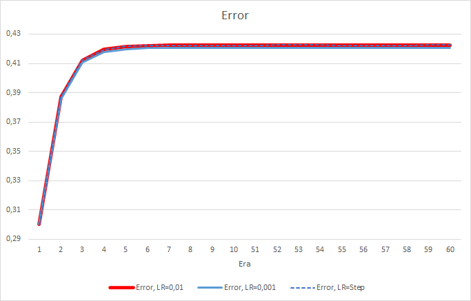
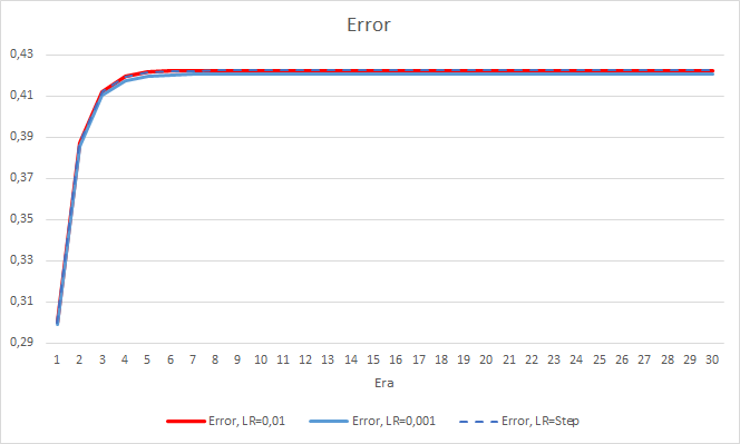
After 5 epochs, the error of all EAs reached the level of 0.42, where it continued to fluctuate for the rest of the time. The error of the EA with the learning rate equal to 0.001 was slightly lower. The differences appeared in the third decimal place (0.420 against 0.422 of the other two EAs).

The error trajectory of the EA with a variable learning rate follows the error line of the EA with a learning factor of 0.01. This is quite expected in the first ten epochs, but there is no deviation when the rate decreases.

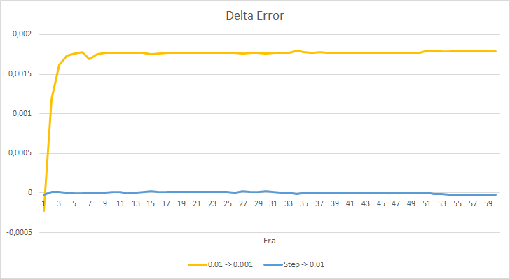
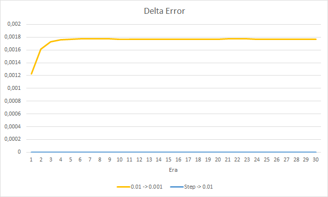
Let us take a closer look at the difference between the errors of the above EAs. Almost throughout the entire experiment, the difference between the errors of EAs with constant learning rates of 0.01 and 0.001 fluctuated around 0.0018. Furthermore, a decrease in the EA's learning rate every 10 epochs has almost no effect and the deviation from the EA with a rate of 0.01 (equal to the initial learning rate) fluctuates around 0.

The obtained error values show that the learning rate of 0.1 is not applicable in our case. The use of a learning rate of 0.01 and below produces similar results with an error of about 42%.

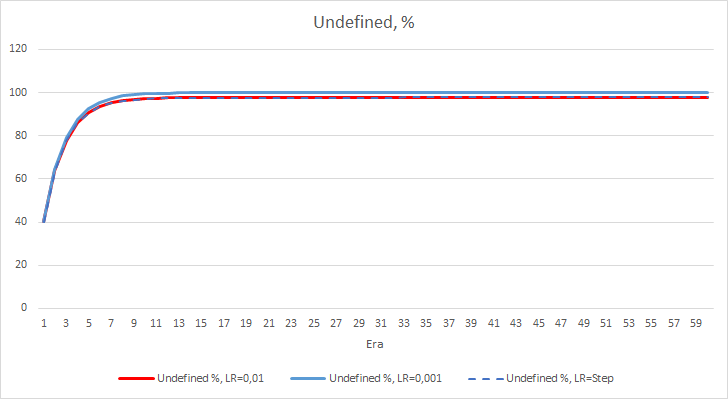
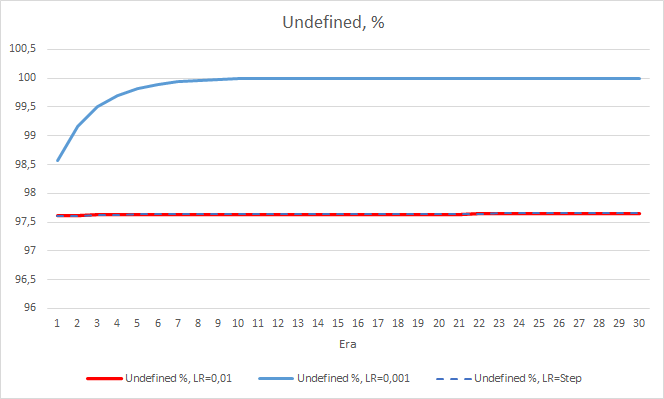
The statistical error of the neural network is quite clear. How will this affect the EA performance? Let us check the number of missed fractals. Unfortunately, all EAs showed bad results during the experiment: they all missed nearly 100% of fractals. Furthermore, an EA with the learning rate of 0.01 determines about 2.5% fractals, while with the rate of 0.001 the EA skipped 100% of fractals. After the 52nd epoch, the EA with the learning rate of 0.01 showed a tendency towards a decrease in the number of skipped fractals. No such tendency was shown by the EA with the variable rate.

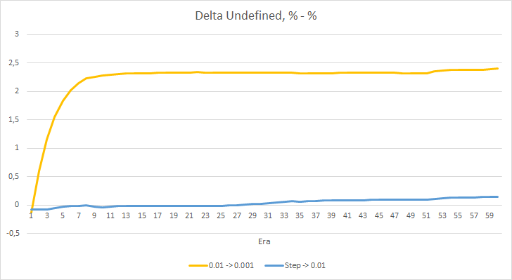
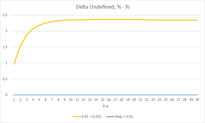
The chart of missing fractal percentage deltas also shows a gradual increase in the difference in favor of the EA with a learning rate of 0.01.

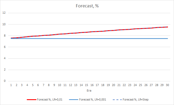
We have considered two neural network performance metrics, and so far the EA with a lower learning rate has a smaller error, but it misses fractals. Now, let us check the third value: "hit" of the predicted fractals.

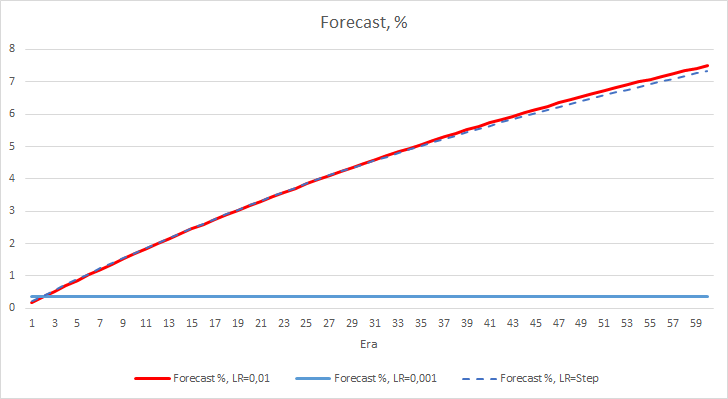
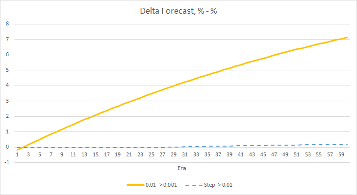
The charts below show a growth of the "hit" percentage in the training of EAs with a learning rate of 0.01 and with a dynamically decreasing rate. The rate of variable growth decreases with a decrease in the learning rate. The EA with the learning rate of 0.001 had the "hit" percentage stuck around 0, which is quite natural because it misses 100% of fractals.

The above experiment shows that the optimal learning rate or training a neural network within our problem is close to 0.01. A gradual decrease in the learning rate did not give a positive result. Perhaps the effect of rate decrease will be different if we decrease it less often than in 10 epochs. Perhaps, results would be better with 100 or 1000 epochs. However, this needs to be verified experimentally.

3. Experiment 2

In the first experiment, the neural network weight matrices were randomly initialized. And therefore, all the EAs had different initial states. To eliminate the influence of randomness on the experiment results, load the weight matrix obtained from the previous experiment with the EA having a learning rate equal to 0.01 into all three EAs and continue training for another 30 epochs.

The new training confirms the earlier obtained results. We see an average error around 0.42 across all three EAs. The EA with the lowest learning rate (0.001) again had a slightly smaller error (with the same difference of 0.0018). The effect of a gradual decrease in the learning rate is practically equal to 0.

As for the percentage of missed fractals, the earlier obtained results are confirmed again. The EA with a lower learning factor approached 100% of missed fractals in 10 epochs, i.e. the EA is unable to indicate fractals. The other two EAs show a value of 97.6%. The effect of a gradual decrease in the learning rate is practically equal to 0.

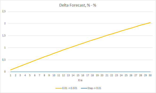
The "hit" percentage of the EA with the learning rate of 0.001 continues to grow gradually. A gradual decrease in the learning rate does not affect this value.

4. Experiment 3

The third experiment is a slight deviation from the main topic of the article. Its idea came about during the first two experiments. So, I decided to share it with you. While observing the neural network training, I noticed that the probability of the absence of a fractal fluctuates around 60-70% and rarely falls below 50%. The probability of emergence of a fractal, wither buy or sell, is around 20-30%. This is quite natural, as there are much less fractals on the chart than there are candlesticks inside trends. Thus, our neural network is overtrained, and we obtain the above results. Almost 100% of fractals are missed, and only rare ones can be caught.

Training the EA with the learning rate of 0.01

To solve this problem, I decided to slightly compensate for the unevenness of the sample: for the absence of a fractal in the reference value, I specified 0.5 instead of 1 when training the network.

            TempData.Add((double)buy);
            TempData.Add((double)sell);
            TempData.Add((double)((!buy && !sell) ? 0.5 : 0));

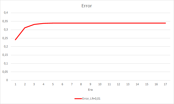
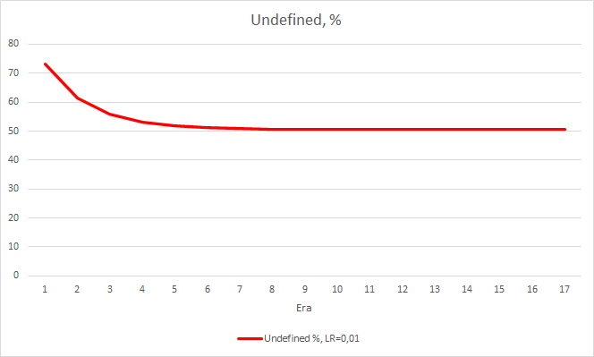
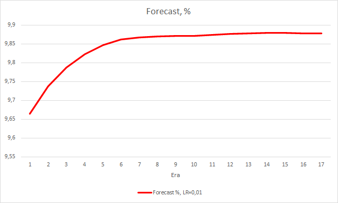
This step produced a good effect. The Expert Advisor running with a learning rate of 0.01 and a weight matrix obtained from previous experiments shows the error stabilization of about 0.34 after 5 training epochs. The share of missed fractals decreased to 51% and the percentage of hits increased to 9.88%. You can see from the chart that the EA generates signals in group and thus shows some certain zones. Obviously, the idea requires additional development and testing. But the results suggest that this approach is quite promising.

$Learning with 0.5 for no fractal$

Conclusions

We have implemented three experiments in this article. The first two experiments have shown the importance of the correct selection of the neural network learning rate. The learning rate affects the overall neural network training result. However, there is currently no clear rule for choosing the learning rate. That is why you will have to select it experimentally in practice.

The third experiment has shown that a non-standard approach to solving a problem can improve the result. But the application of each solution must be confirmed experimentally.

References

Programs used in the article

#	Name	Type	Description
1	Fractal_OCL1.mq5	Expert Advisor	An Expert Advisor with the classification neural network (3 neurons in the output layer) using the OpenCL technology Learning rate = 0.1
2	Fractal_OCL2.mq5	Expert Advisor	An Expert Advisor with the classification neural network (3 neurons in the output layer) using the OpenCL technology Learning rate = 0.01
3	Fractal_OCL3.mq5	Expert Advisor	An Expert Advisor with the classification neural network (3 neurons in the output layer) using the OpenCL technology Learning rate = 0.001
4	Fractal_OCL_step.mq5	Expert Advisor	An Expert Advisor with the classification neural network (3 neurons in the output layer) using the OpenCL technology Learning rate with a 10x decrease from 0.01 every 10 epochs
5	NeuroNet.mqh	Class library	A library of classes for creating a neural network
6	NeuroNet.cl	Code Base	OpenCL program code library