Neural networks made easy (Part 3): Convolutional networks
Dmitriy Gizlyk | 11 December, 2020
Contents
- Introduction
- 1. Distinctive features of convolutional neural networks
- 2. Principles of training neurons in convolutional layers
- 3. Building a convolutional neural network
- 3.1. Base class of neurons
- 3.2. Subsampling layer element
- 3.3. Convolutional layer element
- 3.4. Creating a convolutional neural network class
- 4. Testing
- Conclusion
- List of references
- Programs used in the article
Introduction
As a continuation of the neural network topic, I propose considering convolutional neural networks. These neural networks are usually applied in problems related to object recognition in photo and video images. Convolutional neural networks are believed to be resistant to zooming, changing angles and other spatial image distortions. Their architecture allows recognizing objects equally successfully anywhere in the scene. When applied to trading, I want to use convolutional neural networks to improve the recognition of trading patterns on a price chart.
1. Distinctive features of convolutional neural networks
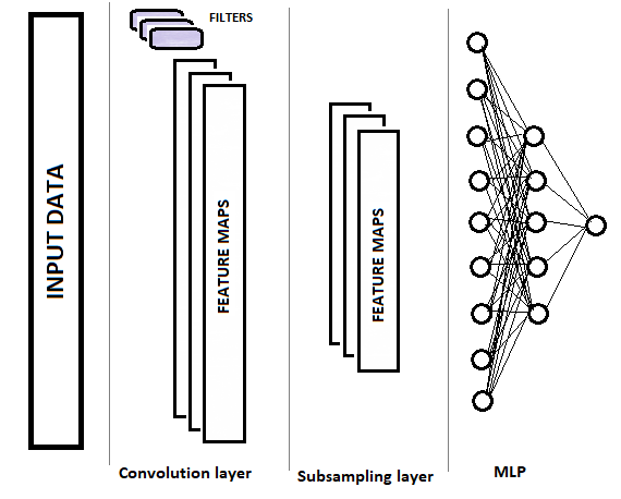
Convolutional networks, in comparison with a fully connected perceptron, have two new layer types: convolutional (filter) and subsampling. These layers alternate with the purpose of selecting the main components and eliminating noises in source data, while reducing data dimension (volume). This data is then input into a fully connected perceptron for decision making. The structure of a convolutional neural network is shown graphically in the figure below. Depending on the tasks, we can use sequentially several groups of alternating convolutional and subsample layers.
1.1. Convolutional layer
The convolution layer is responsible for recognizing objects in the source data array. This layer performs sequential operations of mathematical convolution of the original data, with a small pattern (filter) acting as the convolution kernel.
Convolution is a functional analysis operation on two functions (f and g) that produces a third function corresponding to the cross-correlation function f(x) and g(-x). The convolution operation can be interpreted as the "similarity" of one function with a reversed and shifted copy of another (Wikipedia).
In other words, the convolutional layer searches for a pattern element in the entire original sample. At each iteration, the template is shifted along the initial data array with a given step, which size can be from "1" up to the pattern size. If the offset step size is less than the pattern size, such a convolution is called overlapping.
The convolution operation produces an array of features showing the "similarity" of the original data with the required pattern at each iteration. Activation functions are used to normalize data. The resulting array size will be less than the original data array. The number of such arrays is equal to the number of filters.

An important point is that the patterns are not specified when designing a neural network, but they are selected in the learning process.
1.2. Subsampling layers
The next subsampling layer is used to reduce the dimension of the feature array and to filter noise. The use of this iteration stems from the assumption that the presence of similarity between the original data and the pattern is primary, while the exact coordinates of the feature in the original data array are not so important. This provides a solution to the scaling problem, because it allows some variability in the distance between the desired objects.
At this stage, the data is compacted by keeping the maximum or average value within a given "window". Thus, only one value is saved for each data "window". The operations are performed iteratively, and the window is shifted by a given step at each new iteration. Data compaction is performed separately for each feature array.
Subsample layers with a window and a step equal to 2 are often used - this allows to halve the dimension of the feature array. However, actually larger windows can be used, while compaction iterations can be performed with overlapping (when the step size is less than the window size) or without out.
The subsample layer outputs feature arrays of a smaller dimension.
Depending on the complexity of problems, it is possible to use one or more groups from the convolutional and subsample layer after the subsample layer. Their construction principles and functionality correspond to the above described layer. In the general case, after one or several groups of convolution + compaction, the arrays of features obtained for all filters are collected into a single vector and fed into a multilayer perceptron for the neural network to make a decision (the construction of the multilayer perceptron is described in detail in first part of this article series).
2. Principles of training neurons in convolutional layers
Convolutional neural networks are trained by the back propagation method which was discussed in previous articles. This is one of the supervised learning methods. It consists in descending the error gradient from the output layer of neurons, through the hidden layers, to the input layer of neurons, with weight correction towards the antigradient.
Multilayer perceptron training was explained in the first article, therefore I will not provide an explanation here. Let us consider the training of subsample and convolutional layer neurons.
In the subsample layer, the error gradient is calculated for each feature array element, similarly to the gradients of neurons in a fully connected perceptron. The algorithm for transferring the gradient to the previous layer depends on the applied compaction operation. If only the maximum value is used, the entire gradient is fed to the neuron with the maximum value (a zero gradient is set for all other elements within the compaction window). If the operation of averaging within the window is used, then the gradient is evenly distributed to all elements within the window.
The compaction operation does not use weights, that is why nothing is adjusted in the learning process.
Calculations are somewhat more complex when training the neurons of the convolutional layer. The error gradient is calculated for each element of the feature array and is fed to the corresponding neurons of the previous layer. The convolutional layer training process is based on convolution and inverse convolution operations.
To pass the error gradient from the subsample layer to the convolutional one, the edges of the array of error gradients obtained from the subsample layer are first supplemented with zero elements, and then the resulting array is convolved with the convolution kernel rotated by 180°. The output is an array of error gradients with the dimension equal to the input data array, in which gradient indices correspond to the index of the corresponding neuron preceding the convoluitonal layer.
The delta of weights is obtained by convolving the matrix of input values with the matrix of error gradients of this layer rotated by 180°. This outputs an array of deltas with a size equal to the convolution kernel. The resulting deltas need to be adjusted for the derivative of the convolutional layer activation function and the learning factor. After that the weights of the convolution kernel are changed by the value of the adjusted deltas.
This may sound pretty hard to understand. I will try to clarify some moments in the detailed code analysis below.
3. Building a convolutional neural network
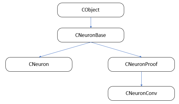
The convolutional neural network will consist of three types of neural layers (convolutional, subsampled and fully connected) with distinctive classes of neurons and different functions for forward and backward pass. At the same time, we need to combine all neurons into a single network and to organize the call of the data processing method which corresponds to the processed neuron. I think the easiest way to organize this process is to use class inheritance and function virtualization.
First, let us build the class inheritance structure.
3.1. Base class of neurons.
In the first article, we have created the CLayer layer class as a descendant of CArrayObj, which is a dynamic array class for storing pointers to CObject class objects. Therefore, all neurons must be inherited from this class. Created the CNeuronBase class based on the CObject class. In the class body, declare variables which are common to all types of neurons, and create templates for the main methods. All methods of the class are declared virtual to enable further redefinition.
class CNeuronBase    :  public CObject
  {
protected:
   double            eta;
   double            alpha;
   double            outputVal;
   uint              m_myIndex;
   double            gradient;
   CArrayCon        *Connections;
//---
   virtual bool      feedForward(CLayer *prevLayer)               {  return false;     }
   virtual bool      calcHiddenGradients( CLayer *&nextLayer)     {  return false;     }
   virtual bool      updateInputWeights(CLayer *&prevLayer)       {  return false;     }
   virtual double    activationFunction(double x)                 {  return 1.0;       }
   virtual double    activationFunctionDerivative(double x)       {  return 1.0;       }
   virtual CLayer    *getOutputLayer(void)                        {  return NULL;      }
public:
                     CNeuronBase(void);
                    ~CNeuronBase(void);
   virtual bool      Init(uint numOutputs, uint myIndex);
//---
   virtual void      setOutputVal(double val)                     {  outputVal=val;    }
   virtual double    getOutputVal()                               {  return outputVal; }
   virtual void      setGradient(double val)                      {  gradient=val;     }
   virtual double    getGradient()                                {  return gradient;  }
//---
   virtual bool      feedForward(CObject *&SourceObject);
   virtual bool      calcHiddenGradients( CObject *&TargetObject);
   virtual bool      updateInputWeights(CObject *&SourceObject);
//---
   virtual bool      Save( int const file_handle);
   virtual bool      Load( int const file_handle)                  {  return(Connections.Load(file_handle)); }
//---
   virtual int       Type(void)        const                       {  return defNeuronBase;                  }
  };
Variable and method names are the same as described earlier. Let us consider methods feedForward(CObject *&SourceObject), сalcHiddenGradients(CObject *&TargetObject) and updateInputWeights(CObject *&SourceObject), in which dispatching for working with fully connected and convolutional layers is performed.
3.1.1. Feed-forward.
The feedForward(CObject *&SourceObject) method is called during a forward pass, for calculating the resulting neuron value. During a forward pass, each neuron in fully connected layers takes the values of all neurons of the previous layer, and must receive the entire previous layer as input. In the convolutional and subsampled layers, only a part of the data related to this filter is fed to the neuron. In the considered method, the algorithm is selected based on the type of the class obtained in the parameters.
First, check the validity of the object pointer obtained in the method parameters.
bool CNeuronBase::feedForward(CObject *&SourceObject)
  {
   bool result=false;
//---
   if(CheckPointer(SourceObject)==POINTER_INVALID)
      return result;
Since class instances cannot be declared inside the selection operator, we need to prepare templates in advance.
   CLayer *temp_l;
   CNeuronProof *temp_n;
Next, in the selection operator, check the type of the object received in the parameters. If a pointer to a layer of neurons is received, then the previous layer is fully connected and, therefore, we need to call a method for working with fully connected layers (described in detail in the first article). If it is a neuron of a convolutional or subsample layer, then first we get a layer of output neurons of this filter and then use a method processing a fully connected layer, to which we should input a layer of neurons of the current filter, and the processing result must be saved in the result variable (further details about the structure of neurons in the convolutional and subsample layers will be provided below). After the operation, exit the method and pass the operation result.
   switch(SourceObject.Type())
     {
      case defLayer:
        temp_l=SourceObject;
        result=feedForward(temp_l);
        break;
      case defNeuronConv:
      case defNeuronProof:
        temp_n=SourceObject;
        result=feedForward(temp_n.getOutputLayer());
        break;
     }
//---
   return result;
  }
3.1.2. Error gradient calculation.
Similarly to a forward pass, a dispatcher was created to call the function calculating an error gradient on the neural network's hidden layers - сalcHiddenGradients(CObject*&TargetObject). The method logic and structure are similar to that described above. First, check the validity of the received pointer. Next, declare variables to store pointers to the corresponding objects. Then, select the appropriate method in the selection function, according to the received object type. Differences occur if a pointer to an element of a convolutional or subsample layer is passed in the parameters. The calculation of the error gradient through such neurons is different and does not apply to all neurons of the previous layer, but only to neurons within the sampling window. That is why the gradient calculation was transferred to these neurons in the calcInputGradients method. Also, there are differences in the methods for calculating by layer or for a specific neuron. Therefore, the required method is called depending on the type of object from which it is called.
bool CNeuronBase::calcHiddenGradients(CObject *&TargetObject)
  {
   bool result=false;
//---
   if(CheckPointer(TargetObject)==POINTER_INVALID)
      return result;
//---
   CLayer *temp_l;
   CNeuronProof *temp_n;
   switch(TargetObject.Type())
     {
      case defLayer:
        temp_l=TargetObject;
        result=calcHiddenGradients(temp_l);
        break;
      case defNeuronConv:
      case defNeuronProof:
        switch(Type())
          {
           case defNeuron:
             temp_n=TargetObject;
             result=temp_n.calcInputGradients(GetPointer(this),m_myIndex);
             break;
           default:
             temp_n=GetPointer(this);
             temp_l=temp_n.getOutputLayer();
             temp_n=TargetObject;
             result=temp_n.calcInputGradients(temp_l);
             break;
          }
        break;
     }
//---
   return result;
  }
The updateInputWeights(CObject *&SourceObject) dispatcher updating all weight is based on the above principles. The full code is available in the attachment.
3.2. Subsampling layer element.
The main building block of the subsample layer is the CNeuronProof class, which inherits from the previously described CNeuronBase base class. One instance of this class will be created for each filter in the subsample layer. Therefore, additional variables (iWindow and iStep) are introduced to store the compaction window size and the shift step. We also add an inner layer of neurons for storing feature arrays, error gradients and, if necessary, weights for passing features to a fully connected perceptron. Also, add a method for receiving a pointer to the inner layer of neurons on demand.
class CNeuronProof : public CNeuronBase
  {
protected:
   CLayer            *OutputLayer;
   int               iWindow;
   int               iStep;

   virtual bool      feedForward(CLayer *prevLayer);
   virtual bool      calcHiddenGradients( CLayer *&nextLayer);

public:
                     CNeuronProof(void){};
                    ~CNeuronProof(void);
   virtual bool      Init(uint numOutputs,uint myIndex,int window, int step, int output_count);
//---
   virtual CLayer   *getOutputLayer(void)  { return OutputLayer;  }
   virtual bool      calcInputGradients( CLayer *prevLayer) ;
   virtual bool      calcInputGradients( CNeuronBase *prevNeuron, uint index) ;
   //--- methods for working with files
   virtual bool      Save( int const file_handle)                         { return(CNeuronBase::Save(file_handle) && OutputLayer.Save(file_handle));   }
   virtual bool      Load( int const file_handle)                         { return(CNeuronBase::Load(file_handle) && OutputLayer.Load(file_handle));   }
   virtual int       Type(void)   const   {  return defNeuronProof;   }
  };
Do not forget to redefine the logic for the virtual functions declared in the base class.
3.2.1. Feed-forward.
The feedForward method is applied to filter out noise and to reduce the dimension of the feature array. In the described solution, the arithmetic mean function is used to compact the data. Let us consider the method code in more detail. At the beginning of the method, check the relevance of the obtained pointer to the previous layer of neurons.
bool CNeuronProof::feedForward(CLayer *prevLayer)
  {
   if(CheckPointer(prevLayer)==POINTER_INVALID)
      return false;
Then loop through all the neurons of the layer obtained in the parameters, with a given step.
   int total=prevLayer.Total()-iWindow+1;
   CNeuron *temp;
   for(int i=0;(i<=total && result);i+=iStep)
     {
In the loop body, create a nested loop for calculating the sum of the output values of the previous layer neurons within the specified compaction window.
      double sum=0;
      for(int j=0;j<iWindow;j++)
        {
         temp=prevLayer.At(i+j);
         if(CheckPointer(temp)==POINTER_INVALID)
            continue;
         sum+=temp.getOutputVal();
        }
After calculating the sum, use the corresponding neuron of the inner layer storing the resulting data, and write the ratio of the obtained sum to the window size to its resulting value. This ratio will be the arithmetic mean for the current compaction window.
      temp=OutputLayer.At(i/iStep);
      if(CheckPointer(temp)==POINTER_INVALID)
         return false;
      temp.setOutputVal(sum/iWindow);
     }
//---
   return true;
  }
After passing through all neurons, the method completes.
3.2.2. Error gradient calculation.
Two methods are created in this class to calculate the error gradient: calcHiddenGradients and calcInputGradients. The first class collects data on the error gradients of the subsequent layer and calculates the gradient for the current layer elements. The second class uses the data obtained in the first method and distributes the error among the previous layer elements.
Again, check the validity of the obtained pointer at the beginning of the calcHiddenGradients method. Additionally, check the state of the inner layer of neurons.
bool CNeuronProof::calcHiddenGradients( CLayer *&nextLayer)
  {
   if(CheckPointer(nextLayer)==POINTER_INVALID || CheckPointer(OutputLayer)==POINTER_INVALID || OutputLayer.Total()<=0)
      return false;
Then, loop through all inner layer neurons and call a method for calculating the error gradient.
   gradient=0;
   int total=OutputLayer.Total();
   CNeuron *temp;
   for(int i=0;i<total;i++)
     {
      temp=OutputLayer.At(i);
      if(CheckPointer(temp)==POINTER_INVALID)
         return false;
      temp.setGradient(temp.sumDOW(nextLayer));
     }
//---
   return true;
  }
Please note that this method works correctly if it is followed by a fully connected layer of neurons. If it is followed by a convolutional or subsampling layer, use the calcInputGradients method of the next layer neuron.
The calcInputGradients method receives a pointer to the previous layer in parameters. Do not forget to check the pointer validity at the method beginning.
bool CNeuronProof::calcInputGradients(CLayer *prevLayer)
  {
   if(CheckPointer(prevLayer)==POINTER_INVALID || CheckPointer(OutputLayer)==POINTER_INVALID)
      return false;
Then check the type of the first element obtained in the layer parameters. If the resulting reference points to a subsample or convolutional layer, then request a reference to the inner layer of neurons corresponding to the filter.
   if(prevLayer.At(0).Type()!=defNeuron)
     {
      CNeuronProof *temp=prevLayer.At(m_myIndex);
      if(CheckPointer(temp)==POINTER_INVALID)
         return false;
      prevLayer=temp.getOutputLayer();
      if(CheckPointer(prevLayer)==POINTER_INVALID)
         return false;
     }
Next, loop through all the neurons of the previous layer, checking the validity of the reference to the processed neuron.
   CNeuronBase *prevNeuron, *outputNeuron;
   int total=prevLayer.Total();
   for(int i=0;i<total;i++)
     {
      prevNeuron=prevLayer.At(i);
      if(CheckPointer(prevNeuron)==POINTER_INVALID)
         continue;
Determine which neurons of the inner layer are affected by the processed neuron.
      double prev_gradient=0;
      int start=i-iWindow+iStep;
      start=(start-start%iStep)/iStep;
      double stop=(i-i%iStep)/iStep+1;
In a loop, calculate the error gradient for the processed neuron and save the result. The method ends after processing all the neurons of the previous layer.
      for(int out=(int)fmax(0,start);out<(int)fmin(OutputLayer.Total(),stop);out++)
        {
         outputNeuron=OutputLayer.At(out);
         if(CheckPointer(outputNeuron)==POINTER_INVALID)
            continue;
         prev_gradient+=outputNeuron.getGradient()/iWindow;
        }
      prevNeuron.setGradient(prev_gradient);
     }
//---
   return true;
  }
The method with same name calculating a separate neuron gradient has a similar structure. The difference is that the external cycle iterating neurons is excluded. Instead, a neuron is called by an index.
Since weights are not used in the subsample layer, the weight updating method can be omitted. If you wish to preserve the structure of neuron classes, you can create an empty method which will create true when called.
The complete code of all methods and functions is available in the attachment.
3.3. Convolutional layer element.
The convolutional layer will be built using the CNeuronConv class objects which will inherit from the CNeuronProof class. I have chosen parametric ReLU as the activation function for this type of neurons. This function is easier to calculate than the hyperbolic tangent which is used in fully connected perceptron neurons. Let us introduce an additional variable param, for calculating the function.
class CNeuronConv  :  public CNeuronProof
  {
protected:
   double            param;   //PReLU param
   virtual bool      feedForward(CLayer *prevLayer);
   virtual bool      calcHiddenGradients(CLayer *&nextLayer);
   virtual double    activationFunction(double x);
   virtual bool      updateInputWeights(CLayer *&prevLayer);
public:
                     CNeuronConv() :   param(0.01) { };
                    ~CNeuronConv(void)             { };
//---
   virtual bool      calcInputGradients(CLayer *prevLayer) ;
   virtual bool      calcInputGradients(CNeuronBase *prevNeuron, uint index) ;
   virtual double    activationFunctionDerivative(double x);
   virtual int       Type(void)   const   {  return defNeuronConv;   }
  };
The forward and backward pass methods are based on algorithms similar to the CNeuron Proof class. The difference is in the use of the activation function and weight coefficients. Therefore, I will not describe them in detail. Let us consider the weight adjustment method updateInputWeights.
The method will receive a pointer to the previous layer of neurons. Again, we check the validity of the pointer and the inner layer state at the method beginning.
bool CNeuronConv::updateInputWeights(CLayer *&prevLayer)
  {
   if(CheckPointer(prevLayer)==POINTER_INVALID || CheckPointer(OutputLayer)==POINTER_INVALID)
      return false;
Next, create a loop through all the weights. Do not forget to check the validity of the received object pointer.
   CConnection *con;
   for(int n=0; n<iWindow && !IsStopped(); n++)
     {
      con=Connections.At(n);
      if(CheckPointer(con)==POINTER_INVALID)
         continue;
After that, calculate the convolution of the input data array with the array of the inner layer error gradients rotated by 180°. This is done in a loop through all elements of the internal layer, multiplied by the input data array elements according to the following scheme:
- the first element of the input data array (with a shift by the number of steps equal to the ordinal number of the weight) multiplied by the last element of the error gradient array,
- the second element of the input data array (with a shift by the number of steps equal to the ordinal number of the weight) multiplied by the second to last element of the error gradient array,
- and so on, until the element with the index equal to the number of elements in the inner layer array with a shift by the number of steps equal to the ordinal number of the weight, is multiplied by the first element of the error gradient array.
Then, find the sum of the resulting products.
      double delta=0;
      int total_i=OutputLayer.Total();
      CNeuron *prev, *out;
      for(int i=0;i<total_i;i++)
        {
         prev=prevLayer.At(n*iStep+i);
         out=OutputLayer.At(total_i-i-1);
         if(CheckPointer(prev)==POINTER_INVALID || CheckPointer(out)==POINTER_INVALID)
            continue;
         delta+=prev.getOutputVal()*out.getGradient();
        }
The calculated sum of the products serves as the basis for adjusting the weights. Adjust weights taking into account the set training speed.
      con.weight+=con.deltaWeight=(delta!=0 ? eta*delta : 0)+(con.deltaWeight!=0 ? alpha*con.deltaWeight : 0);
     }
//---
   return true;
  }
After adjusting all the weights, exit the method.
The CNeuron class is described in detail in the first article. It has not changed much, so I will not provide its description here.
3.4. Create a convolutional neural network class.
Now that all the bricks have been created, we can start building a house. We will create a convolutional neural network class that will combine all types of neurons into a clear structure and will organize the work of our neural network. The first question that arises when creating this class is how to set the required network structure. In the case of a fully connected perceptron, we passed an array of elements with an information about the number of neurons in each layer. Now we need more information to generate the desired network layer. Let us create a small class CLayerDescription for describing the layer construction. This class does not contain any methods (except for the constructor and destructor), and it only includes variables for specifying the type of neurons in the layer, the number of such neurons, the window size and the step for neurons in the convolutional and subsample layers. A pointer to an array of classes with the description of layers will be passed in the parameters of the convolutional network class constructor.
class CLayerDescription    :  public CObject
  {
public:
                     CLayerDescription(void);
                    ~CLayerDescription(void){};
//---
   int               type;
   int               count;
   int               window;
   int               step;
  };
//+------------------------------------------------------------------+
//|                                                                  |
//+------------------------------------------------------------------+
CLayerDescription::CLayerDescription(void)   :  type(defNeuron),
                                                count(0),
                                                window(1),
                                                step(1)
  {}
Let us consider the structure of the CNetConvolution convolutional neural network class. The class contains:
- layers — an array of layers;
- recentAverageError — current network error;
- recentAverageSmoothingFactor — error averaging factor;
- CNetConvolution — class constructor;
- ~CNetConvolution — class destructor;
- feedForward — direct pass method;
- backProp — backward pass method;
- getResults — method for obtaining the results of the last forward pass;
- getRecentAverageError — method for obtaining the current network error;
- Save and Load — methods for saving and loading the previously created and trained method.
class CNetConvolution
  {
public:
                     CNetConvolution(CArrayObj *Description);
                    ~CNetConvolution(void)                     {  delete layers; }
   bool              feedForward( CArrayDouble *inputVals);
   void              backProp( CArrayDouble *targetVals);
   void              getResults(CArrayDouble *&resultVals) ;
   double            getRecentAverageError()                   { return recentAverageError; }
   bool              Save( string file_name, double error, double undefine, double forecast, datetime time, bool common=true);
   bool              Load( string file_name, double &error, double &undefine, double &forecast, datetime &time, bool common=true);
   //---
   static double     recentAverageSmoothingFactor;
   virtual int       Type(void)   const   {  return defNetConv;   }

private:
   CArrayLayer       *layers;
   double            recentAverageError;
  };
Method names and construction algorithms are similar to those for a fully connected perceptron, which were described in first article. Let us dwell only on the main methods of the class.
3.4.1. Convolutional neural network class constructor.
Consider the class constructor. The constructor receives in parameters a pointer to an array of layer descriptions for building a network. So, we need to check the validity of the received pointer, to determine the number of layers and to create a new instance of the layer array.
CNetConvolution::CNetConvolution(CArrayObj *Description)
  {
   if(CheckPointer(Description)==POINTER_INVALID)
      return;
//---
   int total=Description.Total();
   if(total<=0)
      return;
//---
   layers=new CArrayLayer();
   if(CheckPointer(layers)==POINTER_INVALID)
      return;
Next, declare internal variables.
   CLayer *temp;
   CLayerDescription *desc=NULL, *next=NULL, *prev=NULL;
   CNeuronBase *neuron=NULL;
   CNeuronProof *neuron_p=NULL;
   int output_count=0;
   int temp_count=0;
This completes the preparatory work. Let us proceed directly to the cyclic generation of neural network layers. At the beginning of the cycle, read information about the current and next layers.
   for(int i=0;i<total;i++)
     {
      prev=desc;
      desc=Description.At(i);
      if((i+1)<total)
        {
         next=Description.At(i+1);
         if(CheckPointer(next)==POINTER_INVALID)
            return;
        }
      else
         next=NULL;
Count the number of output connections for the layer and create a new instance of the neural layer class. Please note that the number of connections at the layer output should be indicated only before the fully connected layer, otherwise specify zero. This is because convolutional neurons store the input weights themselves, while the subsample layer does not use them at all.
      int outputs=(next==NULL || next.type!=defNeuron ? 0 : next.count);
      temp=new CLayer(outputs);
Then, neurons are generated, with algorithm division according to the type of neurons in the layer. For fully connected layers, a new neuron instance is created and initialized. Please note that for fully connected layers, one more neuron is created, in addition to the number indicated in the description. This neuron will be used as a Bayesian bias.
      for(int n=0;n<(desc.count+(i>0 && desc.type==defNeuron ? 1 : 0));n++)
        {
         switch(desc.type)
           {
            case defNeuron:
              neuron=new CNeuron();
              if(CheckPointer(neuron)==POINTER_INVALID)
                {
                 delete temp;
                 delete layers;
                 return;
                }
              neuron.Init(outputs,n);
              break;
Create a new neuron instance for the convolution layer. Count the number of output elements based on information about the previous layer and initialize the newly created neuron.
            case defNeuronConv:
              neuron_p=new CNeuronConv();
              if(CheckPointer(neuron_p)==POINTER_INVALID)
                {
                 delete temp;
                 delete layers;
                 return;
                }
              if(CheckPointer(prev)!=POINTER_INVALID)
                {
                 if(prev.type==defNeuron)
                   {
                    temp_count=(int)((prev.count-desc.window)%desc.step);
                    output_count=(int)((prev.count-desc.window-temp_count)/desc.step+(temp_count==0 ? 1 : 2));
                   }
                 else
                    if(n==0)
                      {
                       temp_count=(int)((output_count-desc.window)%desc.step);
                       output_count=(int)((output_count-desc.window-temp_count)/desc.step+(temp_count==0 ? 1 : 2));
                      }
                }
              if(neuron_p.Init(outputs,n,desc.window,desc.step,output_count))
                 neuron=neuron_p;
              break;
A similar algorithm is applied to neurons in the subsample layer.
            case defNeuronProof:
              neuron_p=new CNeuronProof();
              if(CheckPointer(neuron_p)==POINTER_INVALID)
                {
                 delete temp;
                 delete layers;
                 return;
                }
              if(CheckPointer(prev)!=POINTER_INVALID)
                {
                 if(prev.type==defNeuron)
                   {
                    temp_count=(int)((prev.count-desc.window)%desc.step);
                    output_count=(int)((prev.count-desc.window-temp_count)/desc.step+(temp_count==0 ? 1 : 2));
                   }
                 else
                    if(n==0)
                      {
                       temp_count=(int)((output_count-desc.window)%desc.step);
                       output_count=(int)((output_count-desc.window-temp_count)/desc.step+(temp_count==0 ? 1 : 2));
                      }
                }
              if(neuron_p.Init(outputs,n,desc.window,desc.step,output_count))
                 neuron=neuron_p;
              break;
           }
After declaring and initializing the neuron, add it to the neural layer.
         if(!temp.Add(neuron))
           {
            delete temp;
            delete layers;
            return;
           }
         neuron=NULL;
        }
Once the cycle generating neurons for the next layer completes, add the layer to the storage. Exit the method after generating all layers.
      if(!layers.Add(temp))
        {
         delete temp;
         delete layers;
         return;
        }
     }
//---
   return;
  }
3.4.2. Convolutional neural network forward propagation method.
The entire operation of the neural network is organized in the feedForward forward pass method. This method receives in parameters the original data for analysis (in our case, this data is information from the price chart and the indicators). First of all, we check the validity of the received reference to the data array and the initialization state of the neural network.
bool CNetConvolution::feedForward(CArrayDouble *inputVals)
  {
   if(CheckPointer(layers)==POINTER_INVALID || CheckPointer(inputVals)==POINTER_INVALID || layers.Total()<=1)
      return false;
Next, declare auxiliary variables and transfer the received external data to the neural network input layer.
   CLayer *previous=NULL;
   CLayer *current=layers.At(0);
   int total=MathMin(current.Total(),inputVals.Total());
   CNeuronBase *neuron=NULL;
   for(int i=0;i<total;i++)
     {
      neuron=current.At(i);
      if(CheckPointer(neuron)==POINTER_INVALID)
         return false;
      neuron.setOutputVal(inputVals.At(i));
     }
After loading the source data into the neural network, run a loop through all the neural layers, from the neural network input of to its output.
   CObject *temp=NULL;
   for(int l=1;l<layers.Total();l++)
     {
      previous=current;
      current=layers.At(l);
      if(CheckPointer(current)==POINTER_INVALID)
         return false;
Inside the launched loop, run a nested loop for each layer, to iterate over all the neurons in the layer and to recalculate their values. Please note that for fully connected neural layers, the value on the last neuron is not recalculated. As mentioned above, this neuron is used as a Bayesian bias and thus only its weight will be used.
      total=current.Total();
      if(current.At(0).Type()==defNeuron)
         total--;
//---
      for(int n=0;n<total;n++)
        {
         neuron=current.At(n);
         if(CheckPointer(neuron)==POINTER_INVALID)
            return false;
Further, the method choice depends on the type of neurons in the previous layer. For fully connected layers, call the forward propagation method, specifying a reference to the previous layer in its parameters.
         if(previous.At(0).Type()==defNeuron)
           {
            temp=previous;
            if(!neuron.feedForward(temp))
               return false;
            continue;
           }
If there was previously a convolutional or subsample layer, check the recalculated neuron type. For a neuron of a fully connected layer, collect the inner layers of all neurons of the previous layer into a single layer and then call the forward propagation method of the current neuron, with a reference to the total layer of neurons specified in the parameters.
         if(neuron.Type()==defNeuron)
           {
            if(n==0)
              {
               CLayer *temp_l=new CLayer(total);
               if(CheckPointer(temp_l)==POINTER_INVALID)
                  return false;
               CNeuronProof *proof=NULL;
               for(int p=0;p<previous.Total();p++)
                 {
                  proof=previous.At(p);
                  if(CheckPointer(proof)==POINTER_INVALID)
                     return false;
                  temp_l.AddArray(proof.getOutputLayer());
                 }
               temp=temp_l;
              }
            if(!neuron.feedForward(temp))
               return false;
            if(n==total-1)
              {
               CLayer *temp_l=temp;
               temp_l.FreeMode(false);
               temp_l.Shutdown();
               delete temp_l;
              }
            continue;
           }
Once the loop though all neurons of this layer has completed, delete the total layer object. Here, it is necessary to delete the layer object without deleting objects of neurons contained in this layer, as the same objects will continue to be used in our convolutional and subsampled layers. This should be done by setting the m_free_mode flag to the false state and then deleting the object.
If this is an element of a convolutional or subsampled layer, then the forward propagation method, passing a pointer to the previous element of the appropriate filter as a parameter.
         temp=previous.At(n);
         if(CheckPointer(temp)==POINTER_INVALID)
            return false;
         if(!neuron.feedForward(temp))
            return false;
        }
     }
//---
   return true;
  }
After iterating over all neurons and layers, exit the method.
3.4.3. Convolutional neural network backward propagation method.
The neural network is trained using the backProp backward propagation method. It implements the method of back error propagation from the output layer of the neural network to its inputs. Therefore, the method receives the actual data in parameters.
At the method beginning, check the validity of the pointer to the pointer value object.
void CNetConvolution::backProp(CArrayDouble *targetVals)
  {
   if(CheckPointer(targetVals)==POINTER_INVALID)
      return;
Then, calculate the root-mean-square error at the output of the neural network's forward pass compared to the actual data, and calculate the error gradients of the output layer neurons.
   CLayer *outputLayer=layers.At(layers.Total()-1);
   if(CheckPointer(outputLayer)==POINTER_INVALID)
      return;
//---
   double error=0.0;
   int total=outputLayer.Total()-1;
   for(int n=0; n<total && !IsStopped(); n++)
     {
      CNeuron *neuron=outputLayer.At(n);
      double target=targetVals.At(n);
      double delta=(target>1 ? 1 : target<-1 ? -1 : target)-neuron.getOutputVal();
      error+=delta*delta;
      neuron.calcOutputGradients(targetVals.At(n));
     }
   error/= total;
   error = sqrt(error);

   recentAverageError+=(error-recentAverageError)/recentAverageSmoothingFactor;
The next step is to organize a backward loop through all neural network layers. Here, we run a nested loop through all neurons of the corresponding layer to recalculate the error gradients of hidden layers neurons.
   CNeuronBase *neuron=NULL;
   CObject *temp=NULL;
   for(int layerNum=layers.Total()-2; layerNum>0; layerNum--)
     {
      CLayer *hiddenLayer=layers.At(layerNum);
      CLayer *nextLayer=layers.At(layerNum+1);
      total=hiddenLayer.Total();
      for(int n=0; n<total && !IsStopped(); ++n)
        {
Similarly to the forward propagation method, the required method for updating the error gradients is selected based on the types of the current neuron and the next layer neurons. If a fully connected layer of neurons follows next, then call the calcHiddenGradients method of the analyzed neuron, passing the pointer to the object of the neural network's next layer in parameters.
         neuron=hiddenLayer.At(n);
         if(nextLayer.At(0).Type()==defNeuron)
           {
            temp=nextLayer;
            neuron.calcHiddenGradients(temp);
            continue;
           }
If this is followed by a convolutional or sub-sample layer, then check the type of the current neuron. For a fully connected neuron, loop though all the filters of the next layer, while launching the error gradient recalculation for each filter for a given neuron. Then sum up the resulting gradients. If the current layer is also convolutional or subsampled, determine the error gradient using the corresponding filter.
         if(neuron.Type()==defNeuron)
           {
            double g=0;
            for(int i=0;i<nextLayer.Total();i++)
              {
               temp=nextLayer.At(i);
               neuron.calcHiddenGradients(temp);
               g+=neuron.getGradient();
              }
            neuron.setGradient(g);
            continue;
           }
         temp=nextLayer.At(n);
         neuron.calcHiddenGradients(temp);
        }
     }
After updating all the gradients, run similar loops with the same branching logic to update the neuron weights. Exit the method after updating the weights.
   for(int layerNum=layers.Total()-1; layerNum>0; layerNum--)
     {
      CLayer *layer=layers.At(layerNum);
      CLayer *prevLayer=layers.At(layerNum-1);
      total=layer.Total()-(layer.At(0).Type()==defNeuron ? 1 : 0);
      int n_conv=0;
      for(int n=0; n<total && !IsStopped(); n++)
        {
         neuron=layer.At(n);
         if(CheckPointer(neuron)==POINTER_INVALID)
            return;
         if(neuron.Type()==defNeuronProof)
            continue;
         switch(prevLayer.At(0).Type())
           {
            case defNeuron:
              temp=prevLayer;
              neuron.updateInputWeights(temp);
              break;
            case defNeuronConv:
            case defNeuronProof:
              if(neuron.Type()==defNeuron)
                {
                 for(n_conv=0;n_conv<prevLayer.Total();n_conv++)
                   {
                    temp=prevLayer.At(n_conv);
                    neuron.updateInputWeights(temp);
                   }
                }
              else
                {
                 temp=prevLayer.At(n);
                 neuron.updateInputWeights(temp);
                }
              break;
            default:
              temp=NULL;
              break;
           }
        }
     }
  }
The complete code of all methods and classes is available in the attachment below.
4. Testing
Let us use the classification Expert Advisor from the second article within this series, in order to test the operation of the convolutional neural network. The purpose of the neural network is to learn to predict a fractal on the current candlestick. For this purpose, feed into the neural network information on the last N candlestick formation and data from 4 oscillators for the same period.
In the neural network's convolutional layer, create 4 filters that will search for patterns in the total candlestick formation data and oscillator readings on the analyzed candlestick. The filter window and step will correspond to the amount of data per candlestick description. In other words, this will compare all the information about each candlestick with a certain pattern and will return the convergence value. This approach allows supplementing of the initial data with new information about the candlesticks (such as adding more indicators for analysis, and so on) without significant performance loss.
The size of the feature array is reduced in the subsampling layer, as well as the results are smoothed by averaging.
The EA itself required a minimum of changes. The change applies to the neural network class, namely the declaration of variables and creation of an instance.
CNetConvolution *Net;
Other changes concern the part that sets the neural network structure in the OnInit function. The test was performed using a network with one convolutional and one subsampling layer each having 4 filters. The structure of fully connected layers has not changed (it was done intentionally to evaluate the impact of convolutional layers on the operation of the entire network).
   Net=new CNetConvolution(NULL);
   ResetLastError();
   if(CheckPointer(Net)==POINTER_INVALID || !Net.Load(FileName+".nnw",dError,dUndefine,dForecast,dtStudied,false))
     {
      printf("%s - %d -> Error of read %s prev Net %d",__FUNCTION__,__LINE__,FileName+".nnw",GetLastError());
      CArrayObj *Topology=new CArrayObj();
      if(CheckPointer(Topology)==POINTER_INVALID)
         return INIT_FAILED;
//---
      CLayerDescription *desc=new CLayerDescription();
      if(CheckPointer(desc)==POINTER_INVALID)
         return INIT_FAILED;
      desc.count=(int)HistoryBars*12;
      desc.type=defNeuron;
      if(!Topology.Add(desc))
         return INIT_FAILED;
//---
      int filters=4;
      desc=new CLayerDescription();
      if(CheckPointer(desc)==POINTER_INVALID)
         return INIT_FAILED;
      desc.count=filters;
      desc.type=defNeuronConv;
      desc.window=12;
      desc.step=12;
      if(!Topology.Add(desc))
         return INIT_FAILED;
//---
      desc=new CLayerDescription();
      if(CheckPointer(desc)==POINTER_INVALID)
         return INIT_FAILED;
      desc.count=filters;
      desc.type=defNeuronProof;
      desc.window=3;
      desc.step=2;
      if(!Topology.Add(desc))
         return INIT_FAILED;
//---
      int n=1000;
      bool result=true;
      for(int i=0;(i<4 && result);i++)
        {
         desc=new CLayerDescription();
         if(CheckPointer(desc)==POINTER_INVALID)
            return INIT_FAILED;
         desc.count=n;
         desc.type=defNeuron;
         result=(Topology.Add(desc) && result);
         n=(int)MathMax(n*0.3,20);
        }
      if(!result)
        {
         delete Topology;
         return INIT_FAILED;
        }
//---
      desc=new CLayerDescription();
      if(CheckPointer(desc)==POINTER_INVALID)
         return INIT_FAILED;
      desc.count=3;
      desc.type=defNeuron;
      if(!Topology.Add(desc))
         return INIT_FAILED;
      delete Net;
      Net=new CNetConvolution(Topology);
      delete Topology;
      if(CheckPointer(Net)==POINTER_INVALID)
         return INIT_FAILED;
      dError=-1;
      dUndefine=0;
      dForecast=0;
      dtStudied=0;
     }
The rest of the Expert Advisor code remained unchanged.
Testing was performed using the EURUSD pair with the H1 timeframe. Two Expert Advisors, one with a convolutional neural network and the other one with fully connected network, were launched simultaneously on different charts of the same symbol, in the same terminal. The parameters of the fully connected layers of the convolutional neural network match the parameters of the fully connected network of the second Expert Advisor, i. e. we have simply added convolutional and subsampled layers to a previously created network.
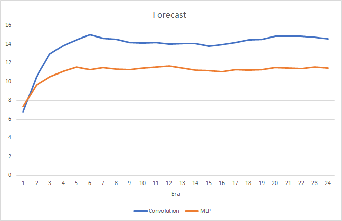
Testing has shown a small performance gain in the convolutional neural network. Despite the addition of two layers, the average training time for one epoch (based on the results of 24 epochs) of a convolutional neural network was 2 hours 4 minutes, and that for a fully connected network was 2 hours 10 minutes.
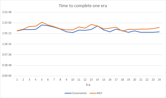
The convolutional neural network shows slightly better results in terms of prediction error and "target hitting".
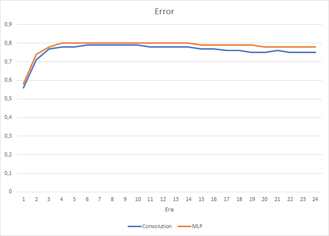
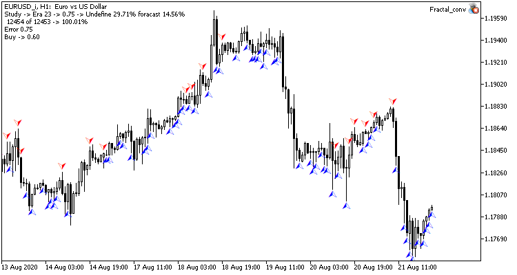
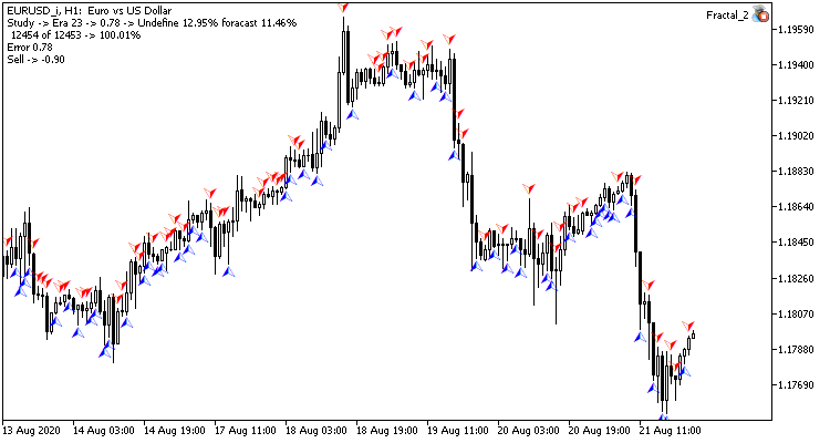
Visually, you can see that signals appear less frequently on the convolutional neural network chart, but they are closer to the target.
Conclusion
In this article, we have examined the possibility of using convolutional neural networks in financial markets. Testing has shown that by using them, we can improve the results of a fully connected neural network. This can be connected with the preprocessing of the data that we feed into the fully connected perceptron. Original data is filtered in the convolutional and subsampled layers to remove noise, which improves the quality of the source data and the quality of the neural network. Furthermore, reduced dimensionality helps to reduce the number of perceptron connections with the original data, which provides an increase in performance.
List of references
Programs used in the article
| # | Issued to | Type | Description |
|---|---|---|---|
| 1 | Fractal.mq5 | Expert Advisor | An Expert Advisor with the regression neural network (1 neuron in the output layer) |
| 2 | Fractal_2.mq5 | Expert Advisor | An Expert Advisor with the classification neural network (3 neurons in the output layer) |
| 3 | NeuroNet.mqh | Class library | A library of classes for creating a neural network (a perceptron) |
| 4 | Fractal_conv.mq5 | Expert Advisor | An Expert Advisor with the convolutional neural network (3 neurons in the output layer) |