Neural networks made easy (Part 2): Network training and testing
Dmitriy Gizlyk | 30 November, 2020
Contents
- Introduction
- 1. Defining the problem
- 2. Neural network model project
- 2.1. Determining the number of neurons in the input layer
- 2.2. Designing hidden layers
- 2.3. Determining the number of neurons in the output layer
- 3. Programming
- 3.1. Preparatory work
- 3.2. Initializing classes
- 3.3. Training the neural network
- 3.4. Improving the gradient calculation method
- 4. Testing
- Conclusion
- Programs used in the article
Introduction
In the previous article entitled Neural Networks Made Easy, we considered the CNet construction principles for working with fully connected neural networks using MQL5. In this article, I am going to demonstrate an example of how to use this class in an Expert Advisor and to evaluate the class in real conditions.
1. Defining the problem
Before we start creating our Expert Advisor, it is necessary to define the goals and objectives that we will set for our new neural network. Of course, the common goal of any Expert Advisor in the financial markets is to make a profit. However, this purpose is very general. We need to set more specific tasks for the neural network. Moreover, we need to understand how to evaluate future results of the neural network.
Another important moment is that the previously created CNet class used principles of supervised learning, and therefore it requires labeled data for the training set.
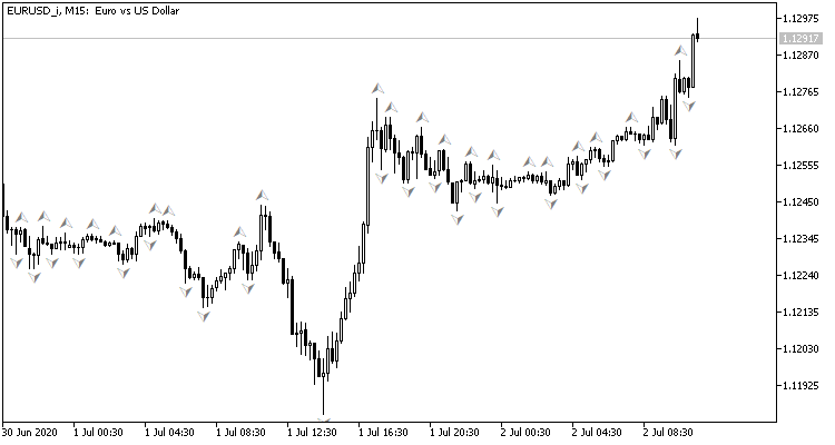
If you look at the price chart, the natural desire would be to execute trading operations at price peaks, which can be shown by the standard Bill Williams fractal indicator. The problem with the indicator is that it determines peaks by 3 candlesticks and always produces a signal delayed by 1 candlestick, which can then turn out to have an opposite signal. What if we set the neural network to determine the pivot points before the third candlestick is formed? This approach would give at least one prior candlestick of movement in the trade direction.
This refers to the training set:
- In the direct pass, we will input the current market situation to the neural network, and it will output an estimate of the probability of pick formation on the last closed candlestick.
- For the reverse pass, after the formation of the next candlestick, we will check if there was a fractal on the previous candlestick and will input the result to adjust the weights.
To evaluate the network operation results, we can use the mean square prediction error, the percentage of correct fractal predictions and the percentage of unrecognized fractals.
Now we need to determine which data should be input into our neural network. Do you remember what you do when you try to assess the market situation based on the chart?
First of all, a novice trader is advised to visually evaluate the trend direction from the chart. Therefore, we must digitize information about price movements and input it into the neural network. I propose to input data about open and close prices, high and low prices, volumes and formation time.
Another popular method to determine the trend is to use oscillator indicators. The use of such indicators is convenient because indicators output normalized data. I decided to use for the experiment four standard indicators: RCI, CCI, ATR and MACD, all with standard parameters. I did not conduct any additional analysis to select indicators and their parameters.
Someone may say that the use of indicators is meaningless, since their data is built from recalculating the price data of candlesticks, which we already input into the neural network. But this is not entirely true. Indicator values are determined by calculating data from several candlestick, which allows a certain expansion of the analyzed sample. The neural network training process will determine how they the affect the result.
To be able to assess the market dynamics, we will input the entire information over a certain historical period into the neural network.
2. Neural network model project
2.1. Determining the number of neurons in the input layer
Here we need to understand the number of neurons in the input layer. To do this, evaluate the initial information on each candlestick and multiply it by the depth of the analyzed history.
There is no need to pre-process the indicator data, as they are normalized and the relevant number of indicator buffers is known (the 4 above indicators all together have 5 values). Therefore, to receive these indicators in the input layer, we need to create 5 neurons for each analyzed candlestick.
The situation is slightly different with candlestick price data. When determining the trend direction and strength visually from a chart, we first analyze candlestick direction and size. Only after that, when we come to determining trend direction and probable pivot points, we pay attention to the price level of the analyzed symbol. Therefore, it is necessary to normalize this data before inputting it to the neural network. I personally input the difference of Close, High and Low prices from the Open price of the described candlestick. In this approach, it is enough to describe three neurons, where the sign of the first neuron determines the candlestick direction.
There are a lot of different materials describing the influence of various time factors on the currency volatility. For example, season, differences in dynamics by weeks and days, as well as European, American and Asian trading sessions affect currency rates in different ways. To analyze such factors, input the candlestick formation month, hour and day of the week into the neural network. I deliberately split the candlestick formation time and date into components, as this enables the neural network to generalize and find dependencies.
Additionally, let's include information about volumes. If your broker provides data on real volumes, indicate these volumes; otherwise specify tick volumes.
Thus, we need 12 neurons to describe each candlestick. By multiplying this number by the analyzed history depth, you will receive the size of the neural network's input layer.
2.2. Designing hidden layers
The next step is to prepare the hidden layers of our neural network. Selection of a network structure (number of layers and neurons) is one of the most difficult tasks. The single layer perceptron is good for the linear separation of classes. Two-layer networks can follow nonlinear boundaries. Three-layer networks enable the description of complex multi-connected areas. When we increase the number of layers, the class of functions is expanded, but this leads to worse convergence and increased cost of training. The number of neurons in each layer must satisfy the expected variability of functions. In fact, very simple networks are not capable of simulating behavior with required accuracy in real conditions, while too complex networks are trained to repeat not only the objective function, but also noise.
In the first article, I mentioned the "5-why" method. Now I propose to continue this experiment and to create a network with 4 hidden layers. I set the number of neurons in the first hidden layer equal to 1000. However, it may also be possible to set up some dependence on the depth of the analyzed period. By using the Pareto rule, we will reduce the number of neurons in each subsequent layer by 70%. In addition, the following limitation will be used: the number of neurons in the hidden layer must not be less than 20.
2.3. Determining the number of neurons in the output layer
The number of neurons in the output layer depends on the task and the approach to its solution. To solve regression problems, it is enough to have one neuron which will produce the expected value. To solve classification problems, we need a number of neurons equal to the expected number of classes - each of the neurons will produce the probability of assigning the original object to each class. In practice, the class of an object is determined by the maximum probability.
For our case, I propose to create 2 neural network variants and to evaluate their applicability for our problem in practice. In the first case, the output layer will have one neuron. Values in the range 0.5...1.0 will correspond to a buy fractal, -0.5...-1.0 will correspond to a sell signal, and values in the range -0.5...0.5 will mean there is no signal. In this solution, the hyperbolic tangent is used as the activation function - it can have output values in the range from -1.0 to +1.0.
In the second case, 3 neurons will be created in the output layer (buy, sell, no signal). In this variant, we will train the neural network to obtain a result in the range 0.0 ... 1.0. Here, the result is the probability of a fractal emergence. The signal will be determined according to the maximum probability, and its direction will be determined according to the index of the neuron with the highest probability.
3. Programming
3.1. Preparatory work
Now, it is time to program. First, add the required libraries:
- NeuroNet.mqh — a library for creating a neural network from the previous article
- SymbolInfo.mqh — standard library for receiving symbol data
- TimeSeries.mqh — standard library for working with time series
- Volumes.mqh — standard library for receiving volume data
- Oscilators.mqh — standard library with oscillator classes
#include "NeuroNet.mqh"
#include <Trade\SymbolInfo.mqh>
#include <Indicators\TimeSeries.mqh>
#include <Indicators\Volumes.mqh>
#include <Indicators\Oscilators.mqh>
The next step is to write the program parameters, with which neural network and indicator parameters will be set.
//+------------------------------------------------------------------+
//|   input parameters                                               |
//+------------------------------------------------------------------+
input int                  StudyPeriod =  10;            //Study period, years
input uint                 HistoryBars =  20;            //Depth of history
ENUM_TIMEFRAMES            TimeFrame   =  PERIOD_CURRENT;
//---
input group                "---- RSI ----"
input int                  RSIPeriod   =  14;            //Period
input ENUM_APPLIED_PRICE   RSIPrice    =  PRICE_CLOSE;   //Applied price
//---
input group                "---- CCI ----"
input int                  CCIPeriod   =  14;            //Period
input ENUM_APPLIED_PRICE   CCIPrice    =  PRICE_TYPICAL; //Applied price
//---
input group                "---- ATR ----"
input int                  ATRPeriod   =  14;            //Period
//---
input group                "---- MACD ----"
input int                  FastPeriod  =  12;            //Fast
input int                  SlowPeriod  =  26;            //Slow
input int                  SignalPeriod=  9;             //Signal
input ENUM_APPLIED_PRICE   MACDPrice   =  PRICE_CLOSE;   //Applied price
Next, declare global variables - their usage will be explained later.
CSymbolInfo         *Symb;
CiOpen              *Open;
CiClose             *Close;
CiHigh              *High;
CiLow               *Low;
CiVolumes           *Volumes;
CiTime              *Time;
CNet                *Net;
CArrayDouble        *TempData;
CiRSI               *RSI;
CiCCI               *CCI;
CiATR               *ATR;
CiMACD              *MACD;
//---
double               dError;
double               dUndefine;
double               dForecast;
double               dPrevSignal;
datetime             dtStudied;
bool                 bEventStudy;
This completes the preparatory work. Now proceed to the initialization of classes.
3.2 Initializing classes
The initialization of classes will be performed in the OnInit function. First, let's create an instance of the CSymbolInfo class for working with symbols and update the data about the chart symbol.
//+------------------------------------------------------------------+
//| Expert initialization function                                   |
//+------------------------------------------------------------------+
int OnInit()
  {
//---
   Symb=new CSymbolInfo();
   if(CheckPointer(Symb)==POINTER_INVALID || !Symb.Name(_Symbol))
      return INIT_FAILED;
   Symb.Refresh();
Then create time series instances. Every time you create a class instance, check if it has been successfully created and initialize it. In case of an error, exit the function with the INIT_FAILED result.
   Open=new CiOpen();
   if(CheckPointer(Open)==POINTER_INVALID || !Open.Create(Symb.Name(),TimeFrame))
      return INIT_FAILED;
//---
   Close=new CiClose();
   if(CheckPointer(Close)==POINTER_INVALID || !Close.Create(Symb.Name(),TimeFrame))
      return INIT_FAILED;
//---
   High=new CiHigh();
   if(CheckPointer(High)==POINTER_INVALID || !High.Create(Symb.Name(),TimeFrame))
      return INIT_FAILED;
//---
   Low=new CiLow();
   if(CheckPointer(Low)==POINTER_INVALID || !Low.Create(Symb.Name(),TimeFrame))
      return INIT_FAILED;
//---
   Volumes=new CiVolumes();
   if(CheckPointer(Volumes)==POINTER_INVALID || !Volumes.Create(Symb.Name(),TimeFrame,VOLUME_TICK))
      return INIT_FAILED;
//---
   Time=new CiTime();
   if(CheckPointer(Time)==POINTER_INVALID || !Time.Create(Symb.Name(),TimeFrame))
      return INIT_FAILED;
Tick volumes are used in this example. If you want to use real volumes, then replace "VOLUME_TICK" with "VOLUME_REAL" when calling the Volumes.Creare method.
After declaring the time series, create instances of classes for working with indicators in a similar way.
   RSI=new CiRSI();
   if(CheckPointer(RSI)==POINTER_INVALID || !RSI.Create(Symb.Name(),TimeFrame,RSIPeriod,RSIPrice))
      return INIT_FAILED;
//---
   CCI=new CiCCI();
   if(CheckPointer(CCI)==POINTER_INVALID || !CCI.Create(Symb.Name(),TimeFrame,CCIPeriod,CCIPrice))
      return INIT_FAILED;
//---
   ATR=new CiATR();
   if(CheckPointer(ATR)==POINTER_INVALID || !ATR.Create(Symb.Name(),TimeFrame,ATRPeriod))
      return INIT_FAILED;
//---
   MACD=new CiMACD();
   if(CheckPointer(MACD)==POINTER_INVALID || !MACD.Create(Symb.Name(),TimeFrame,FastPeriod,SlowPeriod,SignalPeriod,MACDPrice))
      return INIT_FAILED;
Now we can proceed to working directly with the neural network class. First, create a class instance. During CNet class initialization, the constructor parameters pass a reference to an array with the specification of the network structure. Please note that the network training process consumes computational resources and takes much time. Therefore, it would be incorrect to train the network after each start anew. Here is what I do: first I declare the network instance without specifying the structure and try to upload a previously trained network from a local storage (the file name is provided in #define).
#define FileName        Symb.Name()+"_"+EnumToString((ENUM_TIMEFRAMES)Period())+"_"+IntegerToString(HistoryBars,3)+"fr_ea"
...
...
...
...
   Net=new CNet(NULL);
   ResetLastError();
   if(CheckPointer(Net)==POINTER_INVALID || !Net.Load(FileName+".nnw",dError,dUndefine,dForecast,dtStudied,false))
     {
      printf("%s - %d -> Error of read %s prev Net %d",__FUNCTION__,__LINE__,FileName+".nnw",GetLastError());
If previously trained data could not be loaded, message is printed to the log, indicating the error code, and the creation of a new untrained network starts. First, declare an instance of the CArrayInt class, and specify there the structure of the neural network. The number of elements indicates the number of the neural network layers, and the value of the elements indicates the number of neurons in the corresponding layer.
      CArrayInt *Topology=new CArrayInt();
      if(CheckPointer(Topology)==POINTER_INVALID)
         return INIT_FAILED;
As already mentioned earlier, we need 12 neurons in the input layer to describe each candlestick. Therefore, write the product of 12 by the depth of the analyzed history in the first array element.
      if(!Topology.Add(HistoryBars*12))
         return INIT_FAILED;
Then describe the hidden layers. We have determined that there will be 4 hidden layers with 1000 neurons in the first hidden layer. Then the number of neurons will be decreased by 70% in each subsequent layer, but each layer will have at least 20 neurons. Data will be added to an array in a loop.
      int n=1000;
      bool result=true;
      for(int i=0;(i<4 && result);i++)
        {
         result=(Topology.Add(n) && result);
         n=(int)MathMax(n*0.3,20);
        }
      if(!result)
        {
         delete Topology;
         return INIT_FAILED;
        }
Indicate 1 in the output layer for building a regression model.
      if(!Topology.Add(1))
         return INIT_FAILED;
If we used a classification model, we would need to specify 3 for the output neuron.
Next, delete the previously created CNet class instance and create a new one, in which the structure of the neural network to be created is indicated. After creating a new neural network instance, delete the class of the network structure, because it will not be used further.
      delete Net;
      Net=new CNet(Topology);
      delete Topology;
      if(CheckPointer(Net)==POINTER_INVALID)
         return INIT_FAILED;
Set the initial values of the variables to collect statistical data:
- dError - standard deviation (error)
- dUndefine - percentage of undefined fractals
- dForecast - percentage of correctly predicted fractals
- dtStudied — the date of the last training candlestick.
      dError=-1;
      dUndefine=0;
      dForecast=0;
      dtStudied=0;
     }
Don't forget that we need to set the neural network structure, to create a new instance of the neural network class and to initialize the statistical variables only if there is no previously trained neural network to load from local storage.
At the end of the OnInit function, create an instance of the CArrayDouble() class, which will be used to exchange data with the neural network, and start the neural network training process.
I would like to share one more solution here. MQL5 does not have asynchronous function calls. If we explicitly call the learning function from the OnInit function, the terminal will consider the program initialization process unfinished until training is complete. That is why, instead of directly calling the function, we create a custom event, while the training function is called from the OnChartEvent function. When creating an event, specify the training start day in the lparam parameter. This approach allows us to make a function call and to complete the OnInit function.
   TempData=new CArrayDouble();
   if(CheckPointer(TempData)==POINTER_INVALID)
      return INIT_FAILED;
//---
   bEventStudy=EventChartCustom(ChartID(),1,(long)MathMax(0,MathMin(iTime(Symb.Name(),PERIOD_CURRENT,(int)(100*Net.recentAverageSmoothingFactor*(dForecast>=70 ? 1 : 10))),dtStudied)),0,"Init");
//---
   return(INIT_SUCCEEDED);
  }
//+------------------------------------------------------------------+
//| ChartEvent function                                              |
//+------------------------------------------------------------------+
void OnChartEvent(const int id,
                  const long &lparam,
                  const double &dparam,
                  const string &sparam)
  {
//---
   if(id==1001)
     {
      Train(lparam);
      bEventStudy=false;
      OnTick();
     }
  }
Do not forget to clear the memory in the OnDeinit function.
//+------------------------------------------------------------------+
//| Expert deinitialization function                                 |
//+------------------------------------------------------------------+
void OnDeinit(const int reason)
  {
//---
   if(CheckPointer(Symb)!=POINTER_INVALID)
      delete Symb;
//---
   if(CheckPointer(Open)!=POINTER_INVALID)
      delete Open;
//---
   if(CheckPointer(Close)!=POINTER_INVALID)
      delete Close;
//---
   if(CheckPointer(High)!=POINTER_INVALID)
      delete High;
//---
   if(CheckPointer(Low)!=POINTER_INVALID)
      delete Low;
//---
   if(CheckPointer(Time)!=POINTER_INVALID)
      delete Time;
//---
   if(CheckPointer(Volumes)!=POINTER_INVALID)
      delete Volumes;
//---
   if(CheckPointer(RSI)!=POINTER_INVALID)
      delete RSI;
//---
   if(CheckPointer(CCI)!=POINTER_INVALID)
      delete CCI;
//---
   if(CheckPointer(ATR)!=POINTER_INVALID)
      delete ATR;
//---
   if(CheckPointer(MACD)!=POINTER_INVALID)
      delete MACD;
//---
   if(CheckPointer(Net)!=POINTER_INVALID)
      delete Net;
   if(CheckPointer(TempData)!=POINTER_INVALID)
      delete TempData;
  }
3.3. Training the neural network
To train the neural network, create the Train function. Training period start date will be passed to function parameters.
void Train(datetime StartTrainBar=0)
Declare local variables at the beginning of the function:
- count - counting learning epochs
- prev_un - percentage of unrecognized fractals in the previous epoch
- prev_for - percentage of correct fractal "predictions" in the previous epoch
- prev_er - previous epoch error
- bar_time - recalculation bar date
- stop - flag to track the call of forced program termination.
   int count=0;
   double prev_up=-1;
   double prev_for=-1;
   double prev_er=-1;
   datetime bar_time=0;
   bool stop=IsStopped();
   MqlDateTime sTime;
Next, check if the date obtained in the function parameters is not beyond the initially specified training period.
   MqlDateTime start_time;
   TimeCurrent(start_time);
   start_time.year-=StudyPeriod;
   if(start_time.year<=0)
      start_time.year=1900;
   datetime st_time=StructToTime(start_time);
   dtStudied=MathMax(StartTrainBar,st_time);
The neural network training will be implemented in the do-while loop. At the beginning of the loop, recalculate the number of historical bars for training the neural network and save the previous pass statistics.
   do
     {
      int bars=(int)MathMin(Bars(Symb.Name(),TimeFrame,dtStudied,TimeCurrent())+HistoryBars,Bars(Symb.Name(),TimeFrame));
      prev_un=dUndefine;
      prev_for=dForecast;
      prev_er=dError;
      ENUM_SIGNAL bar=Undefine;
Then, adjust the size of the buffers and load the necessary historical data.
      if(!Open.BufferResize(bars) || !Close.BufferResize(bars) || !High.BufferResize(bars) || !Low.BufferResize(bars) || !Time.BufferResize(bars) ||
         !RSI.BufferResize(bars) || !CCI.BufferResize(bars) || !ATR.BufferResize(bars) || !MACD.BufferResize(bars) || !Volumes.BufferResize(bars))
         break;
      Open.Refresh(OBJ_ALL_PERIODS);
      Close.Refresh(OBJ_ALL_PERIODS);
      High.Refresh(OBJ_ALL_PERIODS);
      Low.Refresh(OBJ_ALL_PERIODS);
      Volumes.Refresh(OBJ_ALL_PERIODS);
      Time.Refresh(OBJ_ALL_PERIODS);
      RSI.Refresh(OBJ_ALL_PERIODS);
      CCI.Refresh(OBJ_ALL_PERIODS);
      ATR.Refresh(OBJ_ALL_PERIODS);
      MACD.Refresh(OBJ_ALL_PERIODS);
Update the flag for tracking the forced program termination and declare a new flag indicating that the learning epoch has passed (add_loop).
      stop=IsStopped();
      bool add_loop=false;
Organize a nested training cycle through all historical data. At the beginning of the cycle, check if the end of historical data has been reached. If necessary, change the add_loop flag. Also, display the current state of the neural network training on the chart using comments. This will help to monitor the training process.
      for(int i=(int)(bars-MathMax(HistoryBars,0)-1); i>=0 && !stop; i--)
        {
         if(i==0)
            add_loop=true;
         string s=StringFormat("Study -> Era %d -> %.2f -> Undefine %.2f%% foracast %.2f%%\n %d of %d -> %.2f%% \nError %.2f\n%s -> %.2f",count,dError,dUndefine,dForecast,bars-i+1,bars,(double)(bars-i+1.0)/bars*100,Net.getRecentAverageError(),EnumToString(DoubleToSignal(dPrevSignal)),dPrevSignal);
         Comment(s);
Then check if the predicted system state has been calculated at the previous step of the cycle. If it has, then adjust the weights in the direction of the correct value. To do this, clear the contents of the TempData array, check if the fractal was formed on the previous candlestick, and add a correct value to the TempData array (below is the code for a regression neural network with one neuron in the output layer). After that, call the backProp method of the neural network, passing a reference to the TempData array as a parameter. Update the statistical data in the dForecast (percentage of correctly predicted fractals) and dUndefine (percentage of unrecognized fractals).
         if(i<(int)(bars-MathMax(HistoryBars,0)-1) && i>1 && Time.GetData(i)>dtStudied && dPrevSignal!=-2)
           {
            TempData.Clear();
            bool sell=(High.GetData(i+2)<High.GetData(i+1) && High.GetData(i)<High.GetData(i+1));
            bool buy=(Low.GetData(i+2)<Low.GetData(i+1) && Low.GetData(i)<Low.GetData(i+1));
            TempData.Add(buy && !sell ? 1 : !buy && sell ? -1 : 0);
            Net.backProp(TempData);
            if(DoubleToSignal(dPrevSignal)!=Undefine)
              {
               if(DoubleToSignal(dPrevSignal)==DoubleToSignal(TempData.At(0)))
                  dForecast+=(100-dForecast)/Net.recentAverageSmoothingFactor;
               else
                  dForecast-=dForecast/Net.recentAverageSmoothingFactor;
               dUndefine-=dUndefine/Net.recentAverageSmoothingFactor;
              }
            else
              {
               if(sell || buy)
                  dUndefine+=(100-dUndefine)/Net.recentAverageSmoothingFactor;
              }
           }
After adjusting the neural network weight coefficients, calculate the probability of a fractal emergence at the current historical bar (if i is equal to 0, the probability of a fractal formation on the current bar is calculated). To do this, clear the TempData array and add to it the current data for the neural network input layer. If data adding fails or there is not enough data, exit the loop.
         TempData.Clear();
         int r=i+(int)HistoryBars;
         if(r>bars)
            continue;
//---
         for(int b=0; b<(int)HistoryBars; b++)
           {
            int bar_t=r+b;
            double open=Open.GetData(bar_t);
            TimeToStruct(Time.GetData(bar_t),sTime);
            if(open==EMPTY_VALUE || !TempData.Add(Close.GetData(bar_t)-open) || !TempData.Add(High.GetData(bar_t)-open) || !TempData.Add(Low.GetData(bar_t)-open) ||
               !TempData.Add(Volumes.Main(bar_t)/1000) || !TempData.Add(sTime.mon) || !TempData.Add(sTime.hour) || !TempData.Add(sTime.day_of_week) ||
               !TempData.Add(RSI.Main(bar_t)) ||
               !TempData.Add(CCI.Main(bar_t)) || !TempData.Add(ATR.Main(bar_t)) || !TempData.Add(MACD.Main(bar_t)) || !TempData.Add(MACD.Signal(bar_t)))
                  break;
           }
         if(TempData.Total()<(int)HistoryBars*12)
            break;
After preparing the initial data, run the feedForward method and write the neural network results into the dPrevSignal variable. Below is the code for a regression neural network with one neuron in the output layer. The code for a classification neural network having three neurons in the output layer, is attached below.
         Net.feedForward(TempData);
         Net.getResults(TempData);
         dPrevSignal=TempData[0];
To visualize the operation of the neural network on a chart, display the labels of the predicted fractals for the last 200 candles.
         bar_time=Time.GetData(i);
         if(i<200)
           {
            if(DoubleToSignal(dPrevSignal)==Undefine)
               DeleteObject(bar_time);
            else
               DrawObject(bar_time,dPrevSignal,High.GetData(i),Low.GetData(i));
           }
At the end of the historical data cycle, update the flag of the forced program termination.
         stop=IsStopped();
        }
Once the neural network has been trained on all available historical data, increase the counter of training epochs and save the current state of the neural network to a local file. We will be able to use this when we start the neural network the data next time.
      if(add_loop)
         count++;
      if(!stop)
        {
         dError=Net.getRecentAverageError();
         if(add_loop)
           {
            Net.Save(FileName+".nnw",dError,dUndefine,dForecast,dtStudied,false);
            printf("Era %d -> error %.2f %% forecast %.2f",count,dError,dForecast);
           }
         }
At the end, specify the conditions for exiting the training cycle. Conditions can be as follows: a signal with the probability of reaching the goal above a predetermined level is received; the target error parameter is reached; or when, after a training epoch, the statistical data does not change or changes insignificantly (training stopped at a local minimum). You can define your own conditions for exiting the training process.
     }
   while((!(DoubleToSignal(dPrevSignal)!=Undefine || dForecast>70) || !(dError<0.1 && MathAbs(dError-prev_er)<0.01 && MathAbs(dUndefine-prev_up)<0.1 && MathAbs(dForecast-prev_for)<0.1)) && !stop);
Save the time of the last training candlestick before exiting the training function.
   if(count>0)
     {
      dtStudied=bar_time;
     }
  }
3.4. Improving the gradient calculation method
I would like to draw your attention to the following aspect which I found during the testing process. When training a neural network, in some cases there was an uncontrolled increase in the weight coefficients of hidden layer neurons, due to which maximum allowable variable values were exceeded and, as a consequence, the entire neural network was paralyzed. This happened when the subsequent layer error demanded the neurons to output values beyond the range of possible values of the activation function. The solution which I found was to normalize the target values of neurons. The corrected code of the gradient calculation method is shown below.
void CNeuron::calcOutputGradients(double targetVals)
  {
   double delta=(targetVals>1 ? 1 : targetVals<-1 ? -1 : targetVals)-outputVal;
   gradient=(delta!=0 ? delta*CNeuron::activationFunctionDerivative(targetVals) : 0);
  }
The full code of all methods and functions is available in the attachment.
4. Testing
Test training of the neural network was carried out on the EURUSD pair, on the H1 timeframe. Data on 20 candlesticks was input into the neural network. Training was performed for the last 2 years. To check the results, I launched both two Expert Advisors on two charts of the same terminal: one EA with regression neural network (Fractal - with 1 neuron in the output layer) and classification neural network (Fractal_2 - with 3 neurons in the output layer).
The first training epoch on 12432 bars took 2 hours and 20 minutes. Both EAs performed similarly, with a hit rate of just over 6%.
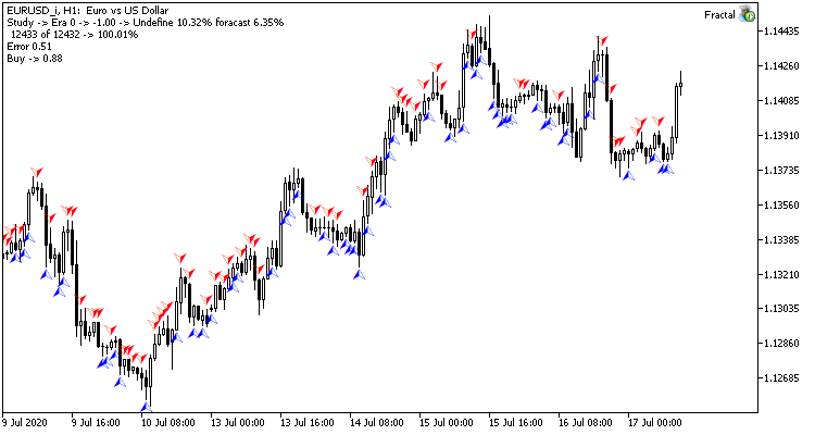
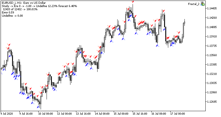
The first epoch is strongly dependent on the weights of the neural network that were randomly selected at the initial stage.
After 35 epochs of training, the difference in statistics increased slightly - the regression neural network model performed better:
| Value | Regression neural network | Classification neural network |
|---|---|---|
| Root mean square error | 0.68 | 0.78 |
| Hit percentage | 12.68% | 11.22% |
| Unrecognized fractals | 20.22% | 24.65% |
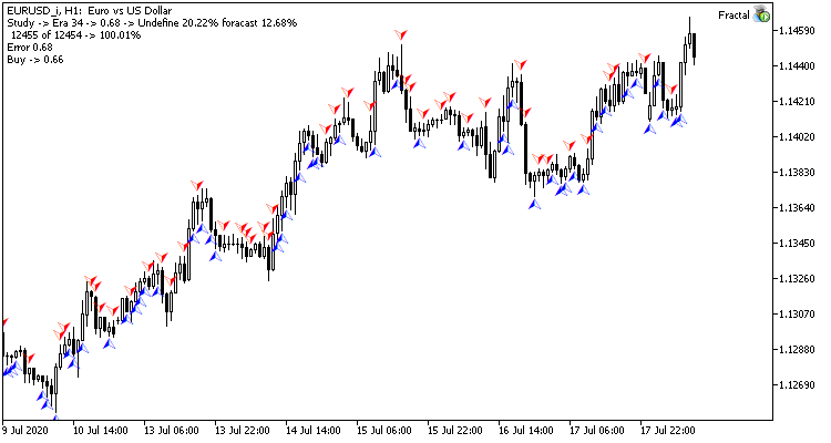
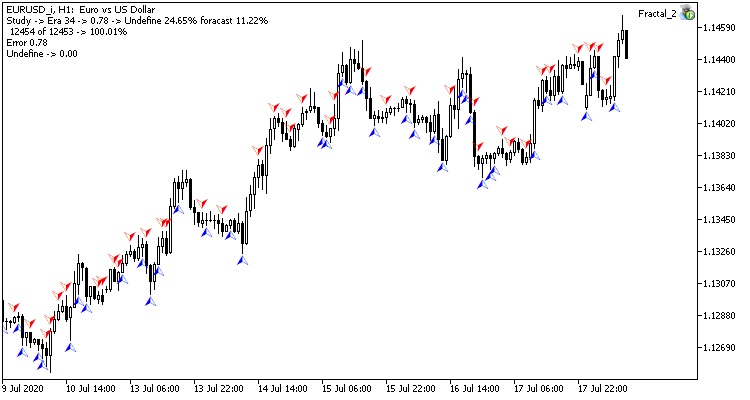
Testing results show that both neural network organization variants generate similar results in terms of training time and prediction accuracy. At the same time, the obtained results show that the neural network needs additional time and resources for training. If you wish to analyze the neural network learning dynamics, please check out the screenshots of each learning epoch in the attachment.
Conclusion
In this article, we considered the process of neural network creation, training and testing. The obtained results show that there is a potential for using this technology. However, the neural network training process consumes a lot of computational resources and takes much time.
Programs used in the article
| # | Issued to | Type | Description |
|---|---|---|---|
| Experts\NeuroNet_DNG\ | |||
| 1 | Fractal.mq5 | Expert Advisor | An Expert Advisor with the regression neural network (1 neuron in the output layer) |
| 2 | Fractal_2.mq5 | Expert Advisor | An Expert Advisor with the classification neural network (3 neurons in the output layer) |
| 3 | NeuroNet.mqh | Class library | A library of classes for creating a neural network (a perceptron) |
| Files\ | |||
| 4 | Fractal | Directory | Contains screenshots showing testing of the regression neural network |
| 5 | Fractal_2 | Directory | Contains screenshots showing testing of the classification neural network |