Neural Networks Made Easy

Table of Contents

• Introduction
• 1. AI network building principles
• 2. The structure of an artificial neuron
• 3. Network training
• 4. Building our own neural network using MQL
• 4.1. Connections
• 4.2. A neuron
• 4.3. Neural network
• Conclusion
• References
• Programs used in the article

Introduction

The Artificial Intelligence is increasingly covering various aspects of our life. A lot of new publications appear, stating that "the neural network was trained to..." However, artificial intelligence is still associated with something fantastic. The idea seems to be very complicated, supernatural and inexplicable. Therefore, such a state-of-the art miracle can only be created by a group of scientists. It seems that a similar program cannot be developed using our home PC. But believe me, it's not that difficult. Let us try to understand what the neural networks are and how they can be applied in trading.

1. AI network building principles

The following neural network definition is provided in Wikipedia:

Artificial neural networks (ANN) are computing systems vaguely inspired by the biological neural networks that constitute animal brains. An ANN is based on a collection of connected units or nodes called artificial neurons, which loosely model the neurons in a biological brain.

That is, a neural network is an entity consisting of artificial neurons, among which there is an organized relationship. These relations are similar to a biological brain.

The figure below shows a simple neural network diagram. Here, circles indicate neurons and lines visualize connections between neurons. Neurons are located in layers which are divided into three groups. Blue indicates the layer of input neurons, which mean an input of source information. Green and blue are output neurons, which output the neural network operation result. Between them are gray neurons forming a hidden layer. 

Despite the layers, the entire network is built of the same neurons having several elements for input signals and only one element for the result. The input data is processed within the neuron and then a simple logical result is output. For example, this can be yes or no. When applied to trading, the result can be output as a trading signal or as a trade direction.

The initial information is input to the input neuron layer, then it is processed and the processing result serves as the source information for the next layer neurons. The operations are repeated from one layer to another until a layer of output neurons is reached. Thus, the initial data is processed and filtered from one layer to another, and after that a result is generated.

Depending on the task complexity and the created models, the number of neurons in each layer can vary. Some network variations may include multiple hidden layers. Such a more advanced neural network can solve more complex problems. However, this would require more computational resources.

Therefore, when creating a neural network model, it is necessary to define the volume of data to be processed and the desired result. This influences the number of required neurons in the model layers.

If we need to input a data array of 10 elements to a neural network, then the input network layer should contain 10 neurons. This will enable the acceptance of all the 10 elements of the data array. Extra input neurons will be excessive.

The quality of output neurons is determined by the expected result. To obtain an unambiguous logical result, one output neuron is enough. If you wish to receive answers to several questions, create one neuron for each of the questions.

Hidden layers serve as an analytical center which processes and analyzes the received information. Therefore, the number of neurons in the layer depends on the variability of the previous-layer data, i.e. each neuron suggests a certain hypothesis of events.

The number of hidden layers is determined by a causal relationship between the source data and the expected result. For example, if we wish to create a model for the "5 why" technique, a logical solution is to use 4 hidden layers, which together with the output layer will make it possible to pose 5 questions to the source data.

Summary:

• a neural network is built of the same neurons, therefore, one class of neurons is enough to build a model;
• neurons in the model are organized in layers;
• data flow in the neural network is implemented as a serial data transmission though all layers of the model, from input neurons to output neurons;
• the number of input neurons depends on the amount of data analyzed per pass, while the number if output neurons depends on the resulting data amount;
• since a logical result is formed at the output, the questions given to the neural network should provide for the possibility to give an unambiguous answer.

2. The structure of an artificial neuron

Now that we have considered the neural network structure, let us move on to the creation of an artificial neuron model. All mathematical calculations and decision making are performed inside this neuron. A question arises here: How can we implement many different solutions based on the same source data and using the same formula? The solution is in changing the connections between neurons. A weight coefficient is determined for each connection. This weight sets how much influence the input value will have on the result.

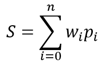
The mathematical model of a neuron consists of two functions. The products of the input data by their weight coefficients are summarized first.

Based on the received value, the result is calculated in the so-called activation function. In practice, different variants of the activation function are used. The most frequently used ones are as follows:

• Sigmoid function — the range of return values from "0" to "1"
• Hyperbolic tangent — the range of return values from "-1" to "1" 

The choice of the activation function depends on the problems being solved. For example, if we expect a logical answer as a result of source data processing, a sigmoid function is preferred. For trading purposes, I prefer to use the hyperbolic tangent. Value "-1" corresponds to the sell signal, "1" corresponds to the buy signal. A medium result indicates uncertainty.

3. Network training

As mentioned above, the result variability of each neuron and of the entire neural network depends on the selected weights for the connections between neurons. The weight selection problem is called neural network learning.

A network can be trained following various algorithms and method:

• Supervised learning;
• Unsupervised learning;
• Reinforcement learning.

The learning method depends in source data and tasks set for the neural network.

Supervised learning is used when there is a sufficient set of initial data with the corresponding correct answers to the questions posed. During the learning process, initial data are input into the network and the output is verified with the known correct answer. After that weights are adjusted to reduce the error.

Unsupervised learning is used when there is a set of initial data without the corresponding correct answers. In this method, the neural network searches for similar data sets and allows dividing source data into similar groups.

Reinforcement learning is used when there are no correct answers, but we understand the desired result. During the learning process, source data is input into the network, which then tries to solve the problem. After verifying the result, a feedback is sent as a certain reward. During learning, the network tries to receive the maximum reward.

In this article we will use supervised learning. As an example, I use the back propagation algorithm. This approach enables continuous neural network training in real time.

The method is based on the use of the output neural network error for the correction of its weights. The learning algorithm consists of two stages. Firstly, based on input data the network calculates the resulting value, which is then verified with the reference value and an error is calculated. Next, a reverse pass is performed, with the propagation of error from the network output to its inputs, with the adjustment of all weighting factors. This is an interactive approach and the network is trained step by step. After learning using historical data, the network can be further trained in the online mode.

The back propagation method uses stochastic gradient descent, which allows reaching an acceptable error minimum. The possibility to further train the network in the online mode allows maintaining this minimum level over a long time interval.

4. Building our own neural network using MQL

Now let us move on to the practical part of the article. For a better visualization of neural network (NN) operation, we will create an example using only the MQL5 language, without any third-party libraries. Let us start with the creation of classes storing data about elementary connections between neurons.

4.1. Connections

Firstly, create the СConnection class to store the weight coefficient of one connection. It is created as the CObject class child. The class will contain two double type variables: 'weight' to store the weight and deltaWeight, in which we will store the value of the last wight change (used in learning). To avoid the need to use additional methods for working with variables, let is make them public. Initial values for the variables are set in the class constructor. 

class СConnection : public CObject
  {
public:
   double            weight;
   double            deltaWeight;
                     СConnection(double w) { weight=w; deltaWeight=0; }
                    ~СConnection(){};
   //--- methods for working with files
   virtual bool      Save(const int file_handle);
   virtual bool      Load(const int file_handle);
  };

To enable saving of further information about connections, let us create method for saving data to a file (Save) and for reading this data (Load). The methods are based on a classical scheme: file handle is received in method parameters, then verified and the data is written (or read in the Load method).

bool СConnection::Save(const int file_handle)
  {
   if(file_handle==INVALID_HANDLE)
      return false;
//---
   if(FileWriteDouble(file_handle,weight)<=0)
      return false;
   if(FileWriteDouble(file_handle,deltaWeight)<=0)
      return false;
//---
   return true;
  }

The next step is to create an array to store weights: CArrayCon based on CArrayObj. Here we override two virtual methods, CreateElement and Type. The first one will be used to create a new element, and the second one will identify our class.

class CArrayCon  :    public CArrayObj
  {
public:
                     CArrayCon(void){};
                    ~CArrayCon(void){};
   //---
   virtual bool      CreateElement(const int index);
   virtual int       Type(void) const { return(0x7781); }
   };

In the parameters of the CreateElement method, which creates a new element, we will pass the index of this new element. Verify the validity in the method, check size of the data storing array and resize if necessary. Then create a new instance of the СConnection class by giving a random initial weight.

bool CArrayCon::CreateElement(const int index)
  {
   if(index<0)
      return false;
//---
   if(m_data_max<index+1)
     {
      if(ArrayResize(m_data,index+10)<=0)
         return false;
      m_data_max=ArraySize(m_data)-1;
     }
//---
   m_data[index]=new СConnection(MathRand()/32767.0);
   if(!CheckPointer(m_data[index])!=POINTER_INVALID)
      return false;
   m_data_total=MathMax(m_data_total,index);
//---
   return (true);
  }

4.2. A neuron

The next step is to create an artificial neuron. As mentioned earlier, I use the hyperbolic tangent as the activation function for my neuron. The range of resulting values is between "-1" an "1". "-1" indicates a sell signal and "1" means a buy signal.

Similarly to the previous CConnection element, the CNeuron artificial neuron class is inherited from the CObject class. However its structure is a little more complicated. 

class CNeuron  :  public CObject
  {
public:
                     CNeuron(uint numOutputs,uint myIndex);
                    ~CNeuron() {};
   void              setOutputVal(double val) { outputVal=val; }
   double            getOutputVal() const { return outputVal; }
   void              feedForward(const CArrayObj *&prevLayer);
   void              calcOutputGradients(double targetVals);
   void              calcHiddenGradients(const CArrayObj *&nextLayer);
   void              updateInputWeights(CArrayObj *&prevLayer);
   //--- methods for working with files
   virtual bool      Save(const int file_handle)                         { return(outputWeights.Save(file_handle));   }
   virtual bool      Load(const int file_handle)                         { return(outputWeights.Load(file_handle));   }

private:
   double            eta;
   double            alpha;
   static double     activationFunction(double x);
   static double     activationFunctionDerivative(double x);
   double            sumDOW(const CArrayObj *&nextLayer) const;
   double            outputVal;
   CArrayCon         outputWeights;
   uint              m_myIndex;
   double            gradient;
  };

In the class constructor parameters, pass the number of outgoing neuron connections and the ordinal number of the neuron in the layer (will be used for subsequent identification of the neuron). In the method body, set constants, save the received data and create an array of outgoing connections.

CNeuron::CNeuron(uint numOutputs, uint myIndex)  :  eta(0.15), // net learning rate
                                                    alpha(0.5) // momentum  
  {
   for(uint c=0; c<numOutputs; c++)
     {
      outputWeights.CreateElement(c);
     }

   m_myIndex=myIndex;
  }

The setOutputVal and getOutputVal methods are used to access the resulting value of the neuron. This resulting value of the neuron is calculated in the feedForward method. The previous layer of neurons is input as parameters to this method.

void CNeuron::feedForward(const CArrayObj *&prevLayer)
  {
   double sum=0.0;
   int total=prevLayer.Total();
   for(int n=0; n<total && !IsStopped(); n++)
     {
      CNeuron *temp=prevLayer.At(n);
      double val=temp.getOutputVal();
      if(val!=0)
        {
         СConnection *con=temp.outputWeights.At(m_myIndex);
         sum+=val * con.weight;
        }
     }
   outputVal=activationFunction(sum);
  }

The method body contains a loop through all previous-layer neurons. The products of resulting neuron values and weights are also summed in the method body. After calculating the sum, the resulting neuron value is calculated in the activationFunction method (the neuron activation function is implemented as in a separate method).

double CNeuron::activationFunction(double x)
  {
//output range [-1.0..1.0]
   return tanh(x);
  }

The next block of methods is used in NN learning. Create a method to calculate a derivative for the activation function, activationFunctionDerivative. This enables the determining of a required change in the summing function to compensate for the error of the resulting neuron value.

double CNeuron::activationFunctionDerivative(double x)
  {
   return 1/MathPow(cosh(x),2);
  }

Next, create two gradient calculation method for weight adjustment. We need to create 2 methods, because the error of the resulting value is calculated in different ways for the neurons of the output layer and those of hidden layers. For the output layer, the error is calculated as the difference between the resulting and the reference value. For hidden layer neurons, the error is calculated as the sum of gradients of all neurons of the subsequent layer weighted based on weights of connections between the neurons. This calculation is implemented as a separate sumDOW method.

void CNeuron::calcHiddenGradients(const CArrayObj *&nextLayer)
  {
   double dow=sumDOW(nextLayer);
   gradient=dow*CNeuron::activationFunctionDerivative(outputVal);
  }
//+------------------------------------------------------------------+
//|                                                                  |
//+------------------------------------------------------------------+
void CNeuron::calcOutputGradients(double targetVals)
  {
   double delta=targetVals-outputVal;
   gradient=delta*CNeuron::activationFunctionDerivative(outputVal);
  }

The gradient is then determined by multiplying the error by the activation function derivative.

Let us consider in more detail the sumDOW method which determines the neuron error for the hidden layer. The method receives a pointer to the next layer of neurons as parameter. In the method body, first set the 'sum' resulting value to zero, and then implement a loop through all neurons of the next layer and sum the product of neuron gradients and the weight of its connection.

double CNeuron::sumDOW(const CArrayObj *&nextLayer) const
  {
   double sum=0.0;
   int total=nextLayer.Total()-1;
   for(int n=0; n<total; n++)
     {
      СConnection *con=outputWeights.At(n);
      CNeuron *neuron=nextLayer.At(n);
      sum+=con.weight*neuron.gradient;
     }
   return sum;
  }

Once the above preparatory work is complete, we only need to create the updateInputWeights method which will recalculate weights. In my model, a neuron stores outgoing weights, so the weight updating method receives the previous layer of neurons in parameters.

void CNeuron::updateInputWeights(CArrayObj *&prevLayer)
  {
   int total=prevLayer.Total();
   for(int n=0; n<total && !IsStopped(); n++)
     {
      CNeuron *neuron= prevLayer.At(n);
      СConnection *con=neuron.outputWeights.At(m_myIndex);
      con.weight+=con.deltaWeight=eta*neuron.getOutputVal()*gradient + alpha*con.deltaWeight;
     }
  }

The method body contains a loop through all neurons of the previous layer, with the adjustment of weights denoting the influence on the current neuron.

Please note that weight adjustment is performed using two coefficients: eta (to reduce reaction to the current deviation) and alpha (inertia coefficient). This approach allows a certain averaging of the influence of a number of subsequent learning iterations and it filters out noise data.

4.3. Neural network

After creating the artificial neuron, we need to combine the create objects into a single entity, the neural network. The resulting objects must be flexible and must allow the creation of neural networks of different configurations. This will allow us to use the resulting solution for various tasks.

As already mentioned above, a neural network consists of layers of neurons. Therefore, the first step is to combine neurons into a layer. Let's create the CLayer class. The basic methods in it are inherited from CArrayObj.

class CLayer: public CArrayObj
  {
private:
   uint              iOutputs;
public:
                     CLayer(const int outputs=0) { iOutputs=outpus; };
                    ~CLayer(void){};
   //---
   virtual bool      CreateElement(const int index);
   virtual int       Type(void) const { return(0x7779); }
   };

In the parameters of the CLayer class initialization method, set the number of elements of the next layer. Also, let's rewrite two virtual methods: CreateElement (creation of a new neuron of the layer) and Type (object identification method).

When creating a new neuron, specify its index in the method parameters. The validity of the received index is checked in the method body. Then check the size of the array for storing pointers to neuron object instances and increase the array size if necessary. After that create the neuron. If the new neuron instance is created successfully, set its initial value and change the number of objects in the array. Then exit the method with 'true'.

bool CLayer::CreateElement(const uint index)
  {
   if(index<0)
      return false;
//---
   if(m_data_max<index+1)
     {
      if(ArrayResize(m_data,index+10)<=0)
         return false;
      m_data_max=ArraySize(m_data)-1;
     }
//---
   CNeuron *neuron=new CNeuron(iOutputs,index);
   if(!CheckPointer(neuron)!=POINTER_INVALID)
      return false;
   neuron.setOutputVal((neuronNum%3)-1)   
//---
   m_data[index]=neuron;
   m_data_total=MathMax(m_data_total,index);
//---
   return (true);
  }

Using a similar approach, create the CArrayLayer class for storing pointers to our network layers.

class CArrayLayer  :    public CArrayObj
  {
public:
                     CArrayLayer(void){};
                    ~CArrayLayer(void){};
   //---
   virtual bool      CreateElement(const uint neurons, const uint outputs);
   virtual int       Type(void) const { return(0x7780); }
   };

The difference from the previous class appears in the CreateElement method which creates a new array element. In this method parameters, specify the number of neurons in the current and further layers to be created. In the method body, check the number of neurons in the layer. If there are no neurons in the created layer, exit with 'false'. Then check if it is necessary to resize the array storing pointers. After that object instances can be created: create a new layer and implement a loop creating neurons. Check the created object at each step. In case of an error exit with the 'false' value. After creating all elements, save a pointer to the created layer in the array and exit with 'true'.

bool CArrayLayer::CreateElement(const uint neurons, const uint outputs)
  {
   if(neurons<=0)
      return false;
//---
   if(m_data_max<=m_data_total)
     {
      if(ArrayResize(m_data,m_data_total+10)<=0)
         return false;
      m_data_max=ArraySize(m_data)-1;
     }
//---
   CLayer *layer=new CLayer(outputs);
   if(!CheckPointer(layer)!=POINTER_INVALID)
      return false;
   for(uint i=0; i<neurons; i++)
      if(!layer.CreatElement(i))
         return false;
//---
   m_data[m_data_total]=layer;
   m_data_total++;
//---
   return (true);
  }

Creation of separate classes for the layer and the array of layers enable the creation of various neural networks having different configurations, without having to change the classes. This is a flexible entity which allows inputting the desired number of layers and neurons per layer.

Now let's consider the CNet class which creates a neural network.

class CNet
  {
public:
                     CNet(const CArrayInt *topology);
                    ~CNet(){};
   void              feedForward(const CArrayDouble *inputVals);
   void              backProp(const CArrayDouble *targetVals);
   void              getResults(CArrayDouble *&resultVals);
   double            getRecentAverageError() const { return recentAverageError; }
   bool              Save(const string file_name, double error, double undefine, double forecast, datetime time, bool common=true);
   bool              Load(const string file_name, double &error, double &undefine, double &forecast, datetime &time, bool common=true);
//---
   static double     recentAverageSmoothingFactor;
private:
   CArrayLayer       layers;
   double            recentAverageError;
  };

We have already implemented a lot of required work in the above classes, and thus the neural network class itself contains a minimum of variables and methods. The class code contain only two statistical variables for calculating and storing the average error (recentAverageSmoothingFactor and recentAverageError), as well as a pointer to the 'layers' array which contains the network layers.

Let's consider the methods of this class in more detail. A pointer to the int data array is passed in the parameters of the class constructor. The number of elements in the array indicates the number of layers, while each element of the array contains the number of neurons in the appropriate layer. Thus, this universal class can be used to create a neural network of any complexity level.

CNet::CNet(const CArrayInt *topology)
  {
   if(CheckPointer(topology)==POINTER_INVALID)
      return;
//---
   int numLayers=topology.Total();
   for(int layerNum=0; layerNum<numLayers; layerNum++) 
     {
      uint numOutputs=(layerNum==numLayers-1 ? 0 : topology.At(layerNum+1));
      if(!layers.CreateElement(topology.At(layerNum), numOutputs))
         return;
     }
  }

In the method body, check the validity of the passed pointer and implement a loop to create layers in the neural network. A zero value of outgoing connections is specified for the output level.

The feedForward method is used for calculating the neural network value. In the parameters, the method receives an array of input values, based on which the resulting values of the neural network will be calculated.

void CNet::feedForward(const CArrayDouble *inputVals)
  {
   if(CheckPointer(inputVals)==POINTER_INVALID)
      return;
//---
   CLayer *Layer=layers.At(0);
   if(CheckPointer(Layer)==POINTER_INVALID)
     {
      return;
     }
   int total=inputVals.Total();
   if(total!=Layer.Total()-1)
      return;
//---
   for(int i=0; i<total && !IsStopped(); i++) 
     {
      CNeuron *neuron=Layer.At(i);
      neuron.setOutputVal(inputVals.At(i));
     }
//---
   total=layers.Total();
   for(int layerNum=1; layerNum<total && !IsStopped(); layerNum++) 
     {
      CArrayObj *prevLayer = layers.At(layerNum - 1);
      CArrayObj *currLayer = layers.At(layerNum);
      int t=currLayer.Total()-1;
      for(int n=0; n<t && !IsStopped(); n++) 
        {
         CNeuron *neuron=currLayer.At(n);
         neuron.feedForward(prevLayer);
        }
     }
  }

In the method body, check the validity of the receives pointer and of the zero layer of our network. Then, set the received initial values as the resulting values of the zero layer neurons and implement a double loop with a phased recalculation of resulting values of neurons throughout the neural network, from the first hidden layer to the output neurons.

The result is obtained using the getResults method, which contains a loop collecting resulting values from the neurons of the output layer.

void CNet::getResults(CArrayDouble *&resultVals)
  {
   if(CheckPointer(resultVals)==POINTER_INVALID)
     {
      resultVals=new CArrayDouble();
     }
   resultVals.Clear();
   CArrayObj *Layer=layers.At(layers.Total()-1);
   if(CheckPointer(Layer)==POINTER_INVALID)
     {
      return;
     }
   int total=Layer.Total()-1;
   for(int n=0; n<total; n++)
     {
      CNeuron *neuron=Layer.At(n);
      resultVals.Add(neuron.getOutputVal());
     }
  }

The neural network learning process is implemented in the backProp method. The method receives an array of reference values in parameters. In the method body, check the validity of the received array and calculate the mean square error of the resulting layer. Then, in the loop, recalculate the gradients of neurons in all layers. After that, in the last method layer, update the weights of connections between neurons based on the earlier calculated gradients.

void CNet::backProp(const CArrayDouble *targetVals)
  {
   if(CheckPointer(targetVals)==POINTER_INVALID)
      return;
   CArrayObj *outputLayer=layers.At(layers.Total()-1);
   if(CheckPointer(outputLayer)==POINTER_INVALID)
      return;
//---
   double error=0.0;
   int total=outputLayer.Total()-1;
   for(int n=0; n<total && !IsStopped(); n++)
     {
      CNeuron *neuron=outputLayer.At(n);
      double delta=targetVals[n]-neuron.getOutputVal();
      error+=delta*delta;
     }
   error/= total;
   error = sqrt(error);

   recentAverageError+=(error-recentAverageError)/recentAverageSmoothingFactor;
//---
   for(int n=0; n<total && !IsStopped(); n++)
     {
      CNeuron *neuron=outputLayer.At(n);
      neuron.calcOutputGradients(targetVals.At(n));
     }
//---
   for(int layerNum=layers.Total()-2; layerNum>0; layerNum--)
     {
      CArrayObj *hiddenLayer=layers.At(layerNum);
      CArrayObj *nextLayer=layers.At(layerNum+1);
      total=hiddenLayer.Total();
      for(int n=0; n<total && !IsStopped();++n)
        {
         CNeuron *neuron=hiddenLayer.At(n);
         neuron.calcHiddenGradients(nextLayer);
        }
     }
//---
   for(int layerNum=layers.Total()-1; layerNum>0; layerNum--)
     {
      CArrayObj *layer=layers.At(layerNum);
      CArrayObj *prevLayer=layers.At(layerNum-1);
      total=layer.Total()-1;
      for(int n=0; n<total && !IsStopped(); n++)
        {
         CNeuron *neuron=layer.At(n);
         neuron.updateInputWeights(prevLayer);
        }
     }
  }

To avoid the need to retrain the system in case of program restart, let's create the 'Save' method for saving data to a local file and the 'Load' method for loading the saved data from the file.

The full code all the class methods is available in the attachment.

Conclusion

The purpose of this article was to show how a neural network can be created at home. Of course, this is only the tip of the iceberg. The article considers only one of the possible versions, i.e. the perceptron, which was introduced by Frank Rosenblatt back in 1957. More than 60 years have passed since the model introduction, and a variety of other models have appeared. However, the perceptron model is still viable and generates good results — you can test the model on your own. Those who wish to go deeper into the idea of the artificial intelligence, should read relevant materials, because it is impossible to cover everything even in a series of articles.

References

1. Wikipedia
2. Perceptron (in Russian)

Programs used in the article

#	Name	Type	Description
1	NeuroNet.mqh	Class library	A library of classes for creating a neural network (a perceptron)