Evaluating the ability of Fractal index and Hurst exponent to predict financial time series
Roman Korotchenko | 11 July, 2019
Introduction
The modern financial market is an example of a "natural" complexly balanced system. On the one hand, the market is pretty chaotic, because it is influenced by a large number of participants. On the other hand, the market is characterized by definite stable processes, which are determined by the market participants' actions. One of econophysics tasks concerns the description of social interaction processes, which form the price dynamics observed on the exchange. Therefore, it is highly desirable to define and present specific properties of financial time series, which will distinguish such data from other natural processes. In modern theories, price series are defined as different-scale fractals (from several minutes to dozens of years).
They show a much more complicated behavior, than many model and natural processes [3]. One of the tools for finding out the details of such behavior is the numerical analysis of the series, the purpose of which is to study the dynamics of the series. The typical algorithms for the reliable evaluation of fractal dimension require large datasets (about 10,000-100,000 samples), which characterize a series over a long time interval, during which the behavior can change, and sometimes it can change repeatedly. For real trading tasks, we need methods to determine the local fractal characteristics of a series. In this article, we will discuss and demonstrate a method for determining the fractal dimension of the series of price sequences, using the numerical method described in [1, 2].
The concept of fractal dimension and statistical properties of time series
The fractal dimension estimates how the data set takes up space. There are many methods for estimating the fractal dimension. Their common feature is that volume or area are calculated in the space, in which this set is located. Let us use the example of the time series for the financial instrument, which consists of Close prices {Close(t)}. If the {Close(t)} series levels are independent, there are no clear trends on the symbol chart, while the behavior will be similar to the "white noise". The value of the fractal dimension D will be close to the value of the topological dimension of the plane, in other words D->2. If the {Close(t)} series levels are not independent, the D value will be significantly less than 2, which indicates that the time series has a "memory", i.e. upward and downward trends will be observed at some time intervals, alternating with the undefined periods (Fig. 1).
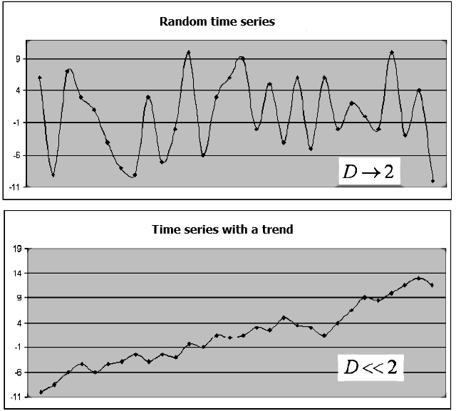
Fig.1. An example of a random series and a series with a trend, and the corresponding fractal dimension
Fractal dimension evaluation methods and their features
There are different methods for calculating the fractal dimension of a time series. Let us consider the evaluation method utilizing the Hurst exponent.
The Hurst exponent H is determined based on the following equation
![]() (1a)
(1a)
where the angle brackets indicate time averaging. The relationship of the Hurst exponent with the fractal dimension is obtained by the method of normalized range or by the R/S analysis based on the following equations
DH = 2-HH = log(R/ S) / log(N / 2) (1b)
where R — max {Close(t)} - min {Close(t)}, i = 1..N is the range of the Close(t) series deviations, S — is the standard deviation of Close(t) values. The method was described in more detail in the article Calculating the Hurst exponent by Dmitry Piskarev.
If the Hurst exponent for the time series is in the range between 0.5 and 1, such a series is considered to be persistent, or trend-resistant, which means that the {Close(t)} series is not random, contains a trend and the behavior of the series can be predicted with a good enough accuracy. The closer the H value to 1, the greater is the correlation between the {Close(t)} series values.
The disadvantage of this method is that a large amount of data (thousands of data series values) is needed in order to obtain a reliable estimate of the Hurst exponent, otherwise the estimates obtained may be incorrect. In addition, the series values must have a normal distribution law, which is not always the case. Since the reliable calculation of both DH and H requires a large representative sample of a large data amount, the series behavior can repeatedly change during the relevant long trading period. In order to link the local dynamics of the analyzed process with the fractal dimension of the observed series, we need to locally determine the D dimension.
Fractal dimension estimation based on minimum covered area
A more efficient method when forecasting econometric series is the one based on the calculation of the minimum coverage dimension
![]() [1, 2]. In 1919,
Hausdorff suggested the following formula for determining a fractal:
[1, 2]. In 1919,
Hausdorff suggested the following formula for determining a fractal:
![]() .
.
where
![]() is the lowest number of balls of radius
is the lowest number of balls of radius
![]() ,
which cover this set. Note that if the original set is in Euclidean space, any other simple shapes (such as cells) can be used for the
set approximation with the geometric factor
,
which cover this set. Note that if the original set is in Euclidean space, any other simple shapes (such as cells) can be used for the
set approximation with the geometric factor
![]() instead of covering the set using balls.
instead of covering the set using balls.
For example, the f(t) function is set in the [a, b] interval. Let us evenly split the interval wm = [a=t0<t1<t2...tm=b], while the
scope of split is defined as
![]() If we cover these sets using, for example, cells sized
If we cover these sets using, for example, cells sized
![]() ,
then if the factor
,
then if the factor
![]() is
decreased, the number of cells
N will increase according to the power law:
is
decreased, the number of cells
N will increase according to the power law:
![]()
where D is the fractal dimension.
When determining the D dimension using the cells method, the surface in which the time series graph is located is
divided into cells of size
![]() ,
and then a calculation is performed to count the number of cells
N(
,
and then a calculation is performed to count the number of cells
N(
![]() ),
to which at least one point of this graph belongs. Then
),
to which at least one point of this graph belongs. Then
![]() changes
and the
N(
changes
and the
N(
![]() )
function graph is plotted in the double logarithmic state. Further, the resulting set of points is approximated using the least square (LS) method. D
is determined based on the line slope.
)
function graph is plotted in the double logarithmic state. Further, the resulting set of points is approximated using the least square (LS) method. D
is determined based on the line slope.
The minimum coverage area of the function graph at this scale, in the [a, b] interval will be equal to the
sum of areas of the rectangles with the base
![]() and
the hight equal to the variation
and
the hight equal to the variation
![]() — the
difference between the maximum and minimum of the
f(t) function at each [ti-1, ti] interval. The minimum coverage area
— the
difference between the maximum and minimum of the
f(t) function at each [ti-1, ti] interval. The minimum coverage area
![]() can
be calculated using the following formula:
can
be calculated using the following formula:
![]() (2)
(2)
where
![]() is
the sum of amplitude variations of function
f(t) in the [a, b] interval. The estimate
is
the sum of amplitude variations of function
f(t) in the [a, b] interval. The estimate
![]() depends
on the selected magnitude. The smaller
depends
on the selected magnitude. The smaller
![]() ,
the more accurate the calculation of
,
the more accurate the calculation of
![]() .
In this case, the value
.
In this case, the value
![]() changes
according to a power lay when
changes
according to a power lay when
![]() changes:
changes:
![]() (3)
(3)
where
![]() .
The value
.
The value
![]() is
called "Dimension of the minimal cover", while index
is
called "Dimension of the minimal cover", while index
![]() is
referred to as the fractal index.
is
referred to as the fractal index.
The dependence of the minimal cover area from different
![]() values
for the time series consisting of 32 observations is shown in Fig. 2.
values
for the time series consisting of 32 observations is shown in Fig. 2.

Fig. 2. Calculating cover area with various values
![]()
Reference [2] states that the fractal dimension which is calculated using the cell covering and covering with rectangle, based on the function variation, coincide. An important property of the algorithm which uses function variations, is its much faster convergence, which allows determining of the time series fractal dimension value locally, using a small set of values.
Applying a logarithm to (3), we obtain the following:
![]() (4)
(4)
To determine
![]() ,
a dependence (3) chart is plotted in double logarithmic coordinates using the least squares (LS) method, and then the tangent of the
straight line angle is determined. Based on expression (4), calculate
,
a dependence (3) chart is plotted in double logarithmic coordinates using the least squares (LS) method, and then the tangent of the
straight line angle is determined. Based on expression (4), calculate
![]() ,
the fractal index, which is the local characteristic of the time series. As is shown in reference [1], the
,
the fractal index, which is the local characteristic of the time series. As is shown in reference [1], the
![]() determining accuracy is
much higher that the accuracy of determining of other fractal characteristics, such as the cellular dimension
determining accuracy is
much higher that the accuracy of determining of other fractal characteristics, such as the cellular dimension
![]() or the dimension
calculated based on the Hurst exponent. In addition, the method has no limitations on the distribution of series
or the dimension
calculated based on the Hurst exponent. In addition, the method has no limitations on the distribution of series
![]() . Reference [1]
also shows that a reliable estimate can be obtained if the time series
. Reference [1]
also shows that a reliable estimate can be obtained if the time series
![]() includes no less than
32 observations. Normally, financial sets have a much longer history. This approach enables the use of the fractal index as a function of
time
includes no less than
32 observations. Normally, financial sets have a much longer history. This approach enables the use of the fractal index as a function of
time
![]() ,
in which each value is determined based on the previous 32 values of the time series
,
in which each value is determined based on the previous 32 values of the time series
![]() .
.
Fig. 3 shows the example of calculation of fractal index
![]() based
on the angle of the approximating straight line. According to the figure, the coefficient of determination of the regression equation
R
2, which approximates the dependence, is equal to 0.96 — this indicates that the fractal index of 0.4544 is calculated
quite accurately for a fragment of a series of 32 points.
based
on the angle of the approximating straight line. According to the figure, the coefficient of determination of the regression equation
R
2, which approximates the dependence, is equal to 0.96 — this indicates that the fractal index of 0.4544 is calculated
quite accurately for a fragment of a series of 32 points.

Fig. 3. Approximation of dependence
![]() in
double logarithmic coordinates and determination of the fractal index
in
double logarithmic coordinates and determination of the fractal index
The fractal dimension can be evaluated using either the cell dimension method or the Hurst index. As an example, let us consider Lukoil stock quotes (MICEX) before the crisis, which happened at the beginning of the century. This time can be interpreted as a stable trend with a gradual increase (persistent series). Fig. 4 shows the results of the fractal dimension evaluation in 1999.

Fig. 4. a) LS approximation of the fractal measure using the cell covering (D=1.1894), b) Log-log plot of the numerical estimate of the Hurst parameter (D=1.6)
The fractal dimension of the series D = 1.18 points to its persistent trendy nature. A value close to one indicates the nearing end of the trend, which happened in 2000-2001. Hurst exponent value H=0.40. Pay attention to the relatively low coefficient of determination R 2= 0.56 with the confidence interval of 0.95. According to formulas (1), the fractal dimension calculated by the Hurst exponent is equal to D = 1.6, which indicates the random behavior of a series and an increased level of stochasticity. However, this does not concern Lukoil stocks in the period of 1999.
Another interesting and illustrative example of the fractal index and Hurst exponent estimation accuracy as of local indicators of time series
is provided in reference [2]. This parameter assessment is more appropriate for the trading tasks related to market analysis of the
operational qualitative and quantitative behavior of time series. The source price series of Alcoa Inc., including 8145 points, was
divided into 8113 overlapping intervals of 32 days each, shifted relative to each other by one day. The following was used as the calculation
accuracy parameters: the width of the confidence interval 95% for
H and
![]() ,
evaluation of accuracy of real points hitting the theoretical line
K = 1- R
2 , where R
2 is the coefficient of determination (of the exactly fall into the line, then R
2=1 and K=0).
,
evaluation of accuracy of real points hitting the theoretical line
K = 1- R
2 , where R
2 is the coefficient of determination (of the exactly fall into the line, then R
2=1 and K=0).
The following values were calculated at each of the 8113 intervals:
- H — Hurst exponent;
-
 —
fractal index;
—
fractal index; -
 — width 95 %
of the confidence interval for
H;
— width 95 %
of the confidence interval for
H; -
 — width 95
% of the confidence interval for
— width 95
% of the confidence interval for
 ;
; -
 - the accuracy
of correspondence of experimental and the obtained straight line for
H;
- the accuracy
of correspondence of experimental and the obtained straight line for
H; -
 - the
accuracy of correspondence of experimental and the obtained straight line for
.
- the
accuracy of correspondence of experimental and the obtained straight line for
.
Typical fragments of graphs of functions
![]() ,
,
![]() and
and
![]() ,
,
![]() ,
built for the intervals, the right value of which coincides with the time t, are shown in Fig. 5a and
5b. It can be seen from these figures, that in most cases index
,
built for the intervals, the right value of which coincides with the time t, are shown in Fig. 5a and
5b. It can be seen from these figures, that in most cases index
![]() is
determined much more accurately, than H.
is
determined much more accurately, than H.
, delta_mu(t)")
Fig. 5a. Typical fragment of the time series of width of confidence intervals created based on the series of Close prices for Alcoa Inc.
, K_mu(t)")
Fig. 5b. The corresponding series fragment for the values showing the accuracy of coincidence of experimental points and the theoretical line, built for the same series
Based on these images, it is possible to conclude that in the overwhelming majority of cases the fractal
index
![]() is
determined much more accurately than H.
is
determined much more accurately than H.
The main advantage of the index
![]() in
relation to other fractal indicators (including in particular the Hurst exponent) is that the corresponding
in
relation to other fractal indicators (including in particular the Hurst exponent) is that the corresponding
![]() value
quickly enters the asymptotic mode. This enables the use of
value
quickly enters the asymptotic mode. This enables the use of
![]() as
the local characteristic by determining the dynamics of the initial process, since the order of the scale for its accurate determining
matches that of the main scale of determining process states. Such states include the relative calm periods (flat) and the long term upward
or downward movement periods (trends). An efficient solution for linking value
as
the local characteristic by determining the dynamics of the initial process, since the order of the scale for its accurate determining
matches that of the main scale of determining process states. Such states include the relative calm periods (flat) and the long term upward
or downward movement periods (trends). An efficient solution for linking value
![]() with
the series behavior, is to add the function
with
the series behavior, is to add the function
![]() as a value
as a value
![]() which
is determined in the minimum interval preceding
t, in which
which
is determined in the minimum interval preceding
t, in which
![]() can
still be calculated with acceptable accuracy.
can
still be calculated with acceptable accuracy.
The correlation of the time series nature and the fractal index
Anyone willing to use an indicator based on the fractal index should know some of its specific features [2].
The behavior of the series defines the
![]() value:
value:
-
 =
0.5 indicates random price walk (Wiener process). Investors behave independently and there is no obvious trend in the
behavior of the price. In this case, we can say that the price has a "normal" stability, because the price is weakly dependent on
external influences, there is no "feedback" and thus there are no arbitrage opportunities.
=
0.5 indicates random price walk (Wiener process). Investors behave independently and there is no obvious trend in the
behavior of the price. In this case, we can say that the price has a "normal" stability, because the price is weakly dependent on
external influences, there is no "feedback" and thus there are no arbitrage opportunities. -
<
0.5 suggests that the price has a higher stability against external influence, which can be connected with the investors'
confidence in the relevant company stability and of absence of any new information in the market. In this case, stock prices
fluctuate within a quite narrow price range. There are still enough sellers when prices grow, as well as there are enough
buyers when prices fall, and their actions get the prices back to the initial range. "Correlation" in this case is negative and
it mitigates stock price changes while preserving stable price behavior.
-
>
0.5 corresponds to reduced price stability. This may indicate the emergence of new information and the reaction to this
information. It can be assumed that all market participants estimate the incoming information approximately equally, and
thus a tendency appears in the price movement corresponding to the information received. Under some conditions, this
situation leads to sharp changes in a stock price.
The fractal index and Hurst exponent are related as
![]() =
1-H, which enables the inheritance of classification variants from chaotic time series:
=
1-H, which enables the inheritance of classification variants from chaotic time series:
- When
=
0.5, H = 0.5 a time series is the Wiener process ("brown" noise). The main property of the process is the absence of memory: series
evolution is not connected with previous values.
- When 0.5 <
<= 1,
0 <= H < 0.5, the process is considered as the "pink" noise. It is characterized by the "negative" memory: if positive
increment was registered in the past, it will be probably followed by a negative increment, and vice versa.
- If 0 <=
<
0.5 , 0.5 < H <=1, the time series is a "black" noise with the positive memory: if positive trend occurred in
the past, it is likely to remain in the future and vice versa.
Indicator for evaluating Fractal index and Hurst exponent
Successful trading on a scale of days, weeks and months is associated with an understanding of the chaotic state of financial time series. Based on the stable evaluation of fractal indexes in short data fragments, we can develop an indicator for stocks (the evolution of which is determined by the will of a large number of people), which will help the trader to identify and forecast financial time series.
The indicator evaluates the fractal index, the confidence interval for it, the values of the coefficient of determination and the Hurst
exponent. The below charts show the aforementioned
![]() ,
,
![]() ,
and
,
and
![]() function graphs.
function graphs.
In the indicator, you can set the length of the time series segment, for which calculation will be performed and the parameter evaluation window will be provided. Upon the indicator launch, the series is calculated along the Close prices while the window is shifted by one count. Since the length of the evaluation window (interval) is equal to the power of two, we can obtain a set of values and evaluate the fractal index by performing the linear approximation of the set.
double CFractalIndexLine::CalculateFractalIndex(const double &series[],const int N0,const int N1,
                                                const double hourSampling,int CountFragmentScale=0)
  {
//- - - - - - - - - - - - - - - - - - - - - - - - - - - - - - - - - - - - - - - - - - - - - - - - - - - - - - - - - - - - - - - - -
// series[] - time series
// N0, N1 - the left and right boundary points of the series[] array fragment, based on which the fractal index will be estimated
// hourSampling - discretization between points in HOURS
// CountFragmentScale - the number of requested scales to form a set of points, for which the fractal index is calculated
//
// RESULT
// the fractal index (Mu), the Hurst index (Hurst), the Confidence interval 95% (ConfInterval[2],
// coefficient of determination (R2det) - the closer to 1, the more accurately the calculation points fall on the approximating line
// determining stability for coefficient KR2 = 1-R2det. The closer to zero, the more accurate the calculated value of Mu
//- - - - - - - - - - - - - - - - - - - - - - - - - - - - - - - - - - - - - - - - - - - - - - - - - - - - - - - - - - - - - - - - -
// 1. Load the internal fragment with values from the time series
   LoadFragment(series,N0,N1,hourSampling);

// 2. Determine the number of cycles to determine the points of the approximating line
   int   nn2 = (int)floor(Nfrgm/2);  // Partition limits - no less than two points
   int npow2 = (int)ipow2(nn2);      // The number of the powers of two in the Possible partitioning limit;

   if(CountFragmentScale==0) CountFragmentScale=npow2; // default

   int Count=fmin(CountFragmentScale,npow2);           // limiting the number of variants of series fragment division
   int NumPartDivide;

   for(int i=0; i<=Count; i++)
     {
      NumPartDivide = (int)pow (2,i);      // Number of pieces in the series fragment division
      CalcAmplVariation(NumPartDivide, i); // Calculating a point for the approximating line model
      i=i;
     }
// 4. Evaluation of the Fractal Index and on the limits of the Index confidence intervals
   Mu=fCalculateConfidenceIntervalMU(LogDeltaScales,LogAmplVariations,Count,ConfInterval,R2det);
   Hurst=1-Mu;		// Hurst exponent
   KR2=1-R2det;

   return Mu;
  }
//----------------------------------------------------------------------------------------------------------------------------------


double CFractalIndexLine::CalcAmplVariation(const int NumPartDivide,int idxAmplVar=-1)
  {
// If idxAmplVar=-1, then index in the array is determined automatically (based on the contribution of the power of two in NumPartDivide)
// ALREADY PREVIOUSLY DONE: copying the fragment, setting the time of discretization of the series IN DAYS
// - - - - - - - - - - - - - - - - - - - - - - - - - - - - - - - - - - - - - - - - - - - - - - -

// 1. DETERMINE THE BORDERS OF INTERVALS CORRESPONDING TO THE SPECIFIC NUMBERS
   int nCheckPoint=0,nIntervalPoints=0; // the number of points to check in one division interval
   double dayDeltaScales=BoundaryArray(NumPartDivide,fragment,0,Nfrgm-1,hSampling,Boundaries,nIntervalPoints);

// 2. GO THROUGH INTERVALS TO DETERMINE LIMIT VALUES OF FUNCTIONS AND OF AMPLITUDE VARIATION
   int countInterval=Boundaries.CountNonEmty();
   int  maxFuncIdx=0,minFuncIdx=0;
   double A,V=0.;

   nCheckPoint=(int)(Boundaries.y[0]-Boundaries.x[0])+1;
   for(int i=0; i<countInterval; i++)
     {
      maxFuncIdx = ArrayMaximum(fragment,(int)Boundaries.x[i],nCheckPoint); // INDEX WITH MAX. VALUE
      minFuncIdx = ArrayMinimum(fragment,(int)Boundaries.x[i],nCheckPoint);
      A = fragment[maxFuncIdx] - fragment[minFuncIdx];
      V = V+A;
      i=i;
     }

// 3. ACCUMULATION OF RESULTS IN STORAGE
   if(idxAmplVar==-1) idxAmplVar=ipow2(NumPartDivide); // index in the storage array

   LogDeltaScales   [idxAmplVar] = log(dayDeltaScales); // log-scale of the current division
   LogAmplVariations[idxAmplVar] = log(V);              // log-Amplitude Variation in the current division scale

   return V;
  }
//--------------------------------------------------------------------------------------------------------------------------------------
CFragmentIndexLine.mqh file fragments execute loops for the calculation of covering area, as it is shown in Fig.2. The sequence of actions in the program is explained through detailed comments.
Demonstration of indicator operation on real data

Fig.6 Close prices of Gazprom and the fractal index evaluation results
The figure shows the correlation of the index values and the behavior of prices. The blue color of the index graph corresponds to the trend state of the system, indicates the trend stability and the ability to predict future behavior. Violet color indicates anti-persistence of the "pink noise" type, which corresponds to "negative" memory and flat. Yellow corresponds to the "Brownian motion", i.e. the movement is random and cannot be predicted.
Conclusions
Local fractal analysis can be interesting in trading for the following purposes:
- Determining of disorder, i.e. of the moment when statistical characteristics of a time series change;
- Prediction of a time series.
It should be taken into account that the scale for determining index
![]() with
a suitable accuracy is two orders of magnitude less than a similar scale for calculating the Hurst exponent H. This difference allows
using index
with
a suitable accuracy is two orders of magnitude less than a similar scale for calculating the Hurst exponent H. This difference allows
using index
![]() as
the local fractal index. That is why it can be considered that index
as
the local fractal index. That is why it can be considered that index
![]() describes
the stability of a time series. Case
describes
the stability of a time series. Case
![]() <0.5
can be interpreted as a trend, and case
<0.5
can be interpreted as a trend, and case
![]() >0.5
can be treated as a flat.
>0.5
can be treated as a flat.
![]() ~
0.5 is considered to be the Brownian motion. Thus, using function
~
0.5 is considered to be the Brownian motion. Thus, using function
![]() we
can classify initial price series and provide basis for forecasts.
we
can classify initial price series and provide basis for forecasts.
List of References
- Dubovikov M.M., Starchenko N.V. Econophysics and fractal analysis of financial time series
- Dubovikov M.M., Starchenko N.V. Econophysics and analysis of financial time series // Collected. "ECONOPHYSICS. Modern physics in search of economic theory"
- Peters, J. Chaos and Order in the Capital Markets A New View of Cycles, Prices and Market Volatility
- Krivonosova
E.K., Pervadchuk V.P., Krivonosova E.A.Comparison of the fractal characteristics of time series of economic indicators
- Starchenko N.V. Local fractal analysis in physical applications.