Grokking market "memory" through differentiation and entropy analysis
Maxim Dmitrievsky | 17 July, 2019
Reason for the approach use and a brief background
A large number of participants in liquid markets, who operate with different investment horizons, produce a lot of market noise. Thus markets have a low signal-to-noise ratio. The situation can be worsened by attempts of integer time series differentiation, which erases the remaining memory and converts quotes to a series characterized by stationarity.
Price series have memory, because each value depends on a long history of price levels. Time series transformations, such as for example the logarithm of increments, crop the memory because they are created based on a limited window length. When transformations to stationarity remove market memory, statisticians use complex mathematical methods to extract the remaining memory. That is why many of the related classical statistical approaches lead to false results.
The concept of long-range dependence
Long-range dependence (LRD), also called long memory or long-range persistence, is a phenomenon which may arise in the analysis of financial time series. This is expressed in the decay rate of the statistical dependence between two prices with an increase in the time interval (or the distance between them). A phenomenon is considered to have a long-range dependence, when the dependence decays slower than the exponential decay. Long-range dependency is also often associated with self-similar processes. For details about LRD (Long-Range Dependence), please read the Wikipedia article.
The problem of stationarity and existence of memory
A common feature of price charts is the non-stationarity: they have a long history of price levels which shift the average price over time. In order to perform a statistical analysis, researchers need to work with price increments (or logarithms of increments), changes in profitability or volatility. These transformations make the time series stationary by removing the memory from price sequences. Although stationarity is a necessary property for statistical conclusions, it is not always necessary to delete the entire memory, since the memory is the basis for the predictive properties of models. For example, equilibrium (stationary) models must contain some memory in order to enable the evaluation of how far the price has moved away from its expected value.
The problem is that price increments are stationary but do not contain memory of the past, while the price series contains the entire amount of available memory but it is non-stationary. The question arises: how to differentiate a time series to make it stationary and at the same time to preserve the maximum possible amount of memory. Therefore we would like to generalize the concept of price increments for considering stationary series in which not all memory is erased. In this case, price increments are not the optimal solution for price transformation, among other available methods.
For this purpose, the concept of fractional differentiation will be introduced. There is a wide range of possibilities between the two extremes: single and zero differentiation. On its one edge, there are fully differentiated prices. Not differentiated prices are at its other edge.
The scope of use of fractional differentiation is wide enough. For example, a differentiated series is usually input into machine learning algorithms. The problem is that it is necessary to display new data in accordance with the available history, which the machine learning model can recognize. In case of a non-stationary series, new data can be located outside the known range of values, due to which the model may operate incorrectly.
The history of fractional differentiation
Almost all methods for the analysis and forecasting of financial time series, described in various scientific articles, present the idea of integer differentiation.
The following questions arise in this connection:
- Why is integer differentiation (say, with a unit lag) optimal?
- Isn't such overdifferentiation one of the reasons why the economic theory is prone to hypothesis of efficient markets?
The concept of fractional differentiation, as applied to time series analysis and forecasting, goes back at least to Hosking. In his article, the family of ARIMA processes was generalized allowing the differentiation degree to have the fractional part. This made sense, because the fractional differentiation process revealed long-range persistence or anti-persistence and thus increased the predictive ability compared to standard ARIMA. This model was called ARFIMA (autoregressive fractionally integrated moving average) or FARIMA. After that, fractional differentiation was sometimes mentioned in articles by other authors, mainly in connection with the calculation method acceleration.
Such models can be useful in modeling long-memory time series, i.e. in cases where deviations from the long-range average decay more slowly than the exponential decay.
The concept of fractional differentiation
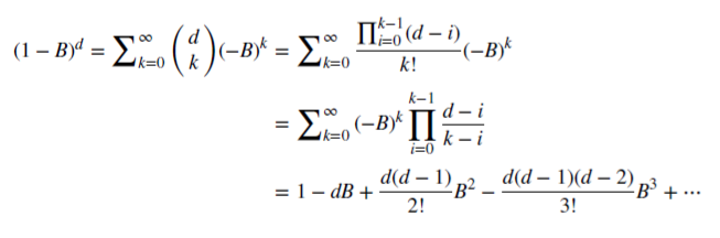
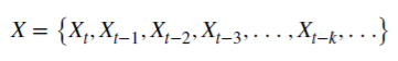
Let us consider the backshift operator (or a lag operator) B, applied to the matrix of real values {Xt}, where B^kXt = Xt−k, for any integer k ≥ 0. For example, (1 − B)^2 = 1 − 2B + B^2, where B^2Xt = Xt−2, consequently, (1 − B)^2Xt = Xt − 2Xt−1 + Xt−2.
Note that (x + y)^n = 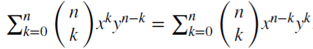 for each positive integer n. For the real number d,
 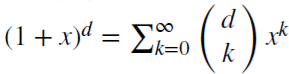 is a binomial series. In the fractional model, d may be a real number with the following formal extension of the binomial series:
Preserving market memory in case of fractional differentiation
Let is see how rational non-negative d can preserve the memory. This arithmetic series consists of a scalar product:
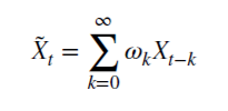
with weights 𝜔
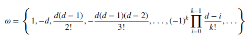
and values X
When d is a positive integer, 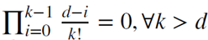 , memory is cropped in this case.
For example, d = 1 is used for calculating increments where 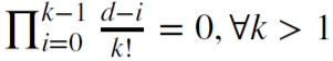 and 𝜔 = {1,−1, 0, 0,…}.
Fractional differentiation for a fixed observation window
Fractional differentiation is usually applied to the entire sequence of a time series. Complexity of calculation is higher in this case, while the shift of the transformed series is negative. Marcos Lopez De Prado in his book Advances in Financial Machine Learning proposed a method of a fixed-width window, in which the sequence of coefficients is discarded when their module (|𝜔k|) becomes less than the specified threshold (𝜏). This procedure has the following advantage over the classical expanding window method: it allows having equal weights for any sequence of the original series, reduces the computational complexity and eliminates the backshift. This conversion allows saving memory about price levels and the noise. The distribution of this transformation is not normal (Gaussian) due to the presence of memory, asymmetry and excess kurtosis, however, it can be stationary.
Demonstration of fractional differentiation process
Let us create a script which will allow you to visually evaluate the effect obtained from the fractional differentiation of the time series. We will create two functions: one for obtaining weights 𝜔 and the other for calculating new values of the series:
//+------------------------------------------------------------------+
void get_weight_ffd(double d, double thres, int lim, double &w[]) {
    ArrayResize(w,1);
    ArrayInitialize(w,1.0);
    ArraySetAsSeries(w,true);

    int k = 1;
    int ctr = 0;
    double w_ = 0;
    while (ctr != lim - 1) {
        w_ = -w[ctr] / k * (d - k + 1);
        if (MathAbs(w_) < thres) break;
        ArrayResize(w,ArraySize(w)+1);
        w[ctr+1] = w_;
        k += 1;
        ctr += 1;
    }
}
//+------------------------------------------------------------------+
void frac_diff_ffd(double &x[], double d, double thres, double &output[]) {
   double w[];
   get_weight_ffd(d, thres, ArraySize(x), w);

   int width = ArraySize(w) - 1;

   ArrayResize(output, width);
   ArrayInitialize(output,0.0);
   ArraySetAsSeries(output,true);
   ArraySetAsSeries(x,true);
   ArraySetAsSeries(w,true);

   int o = 0;
   for(int i=width;i<ArraySize(x);i++) {
      ArrayResize(output,ArraySize(output)+1);

      for(int l=0;l<ArraySize(w);l++)
         output[o] += w[l]*x[i-width+l];
      o++; }
   ArrayResize(output,ArraySize(output)-width);
}
Let us display an animated chart which changes depending on the parameter 0<d<1:
//+------------------------------------------------------------------+
//| Script program start function                                    |
//+------------------------------------------------------------------+
void OnStart()
  {
   for(double i=0.05; i<1.0; plotFFD(i+=0.05,1e-5))
  }
//+------------------------------------------------------------------+
void plotFFD(double fd, double thresh) {
   double prarr[], out[];
   CopyClose(_Symbol, 0, 0, hist, prarr);

   for(int i=0; i < ArraySize(prarr); i++)
      prarr[i] = log(prarr[i]);

   frac_diff_ffd(prarr, fd, thresh, out);
   GraphPlot(out,1); Sleep(500);
}
Here is the result:
Fig. 1. Fractional differentiation 0<d<1
As expected, with an increase in the degree of differentiation d, the charts becomes more stationary, while gradually losing the "memory" of past levels. The weights for the series (the function of the scalar product of weights by price values) remain unchanged during the entire sequence and do not need recalculation.
Creating an indicator based on fractional differentiation
For the convenient use in Expert Advisors, let us create an indicator which we will be able to include, specifying various specified parameters: the degree of differentiation, the size of the threshold for removing excess weights and the depth of the displayed history. I will not post the full indicator code here, so you can view it in the source file.
I will only indicate that the weight calculation function is the same. The following function is used for calculating the indicator buffer values:
frac_diff_ffd(weights, price, ind_buffer, hist_display, prev_calculated !=0);
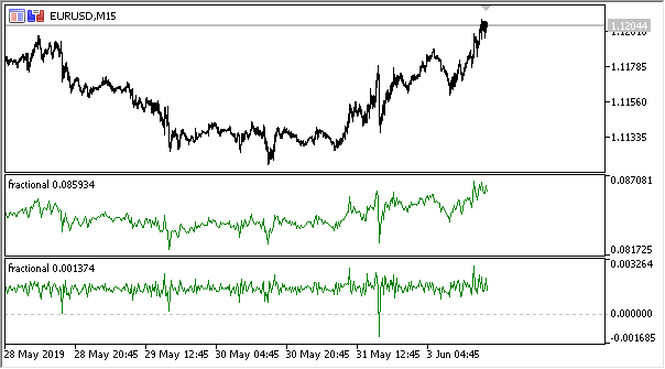
Fig. 2. Fractional differentiation with powers of 0.3 and 0.9
Now we have an indicator which quite accurately explicates the information amount change dynamics in a time series. When the degree of differentiation increases, information is lost and the series becomes more stationary. However, only price level data is lost. What may be left is the periodic cycles which will be the reference point for forecasting. So we are approaching the information theory methods, namely the information entropy, which will help with the assessment of the data amount.
The concept of information entropy
Informational entropy is a concept related to the information theory, which shows how much information is contained in an event. In general, the more specific or deterministic the event, the less information it will contain. More specifically, information is connected with an increase in uncertainty. This concept was introduced by Claude Shannon.
The entropy of a random value can be determined by introducing the concept of distribution of a random X value, which takes a finite number of values:
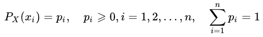
Then the specific information of the event (or of the time series) is defined as follows:
![]()
The entropy estimate can be written as follows:
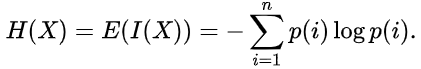
The unit of measurement of the information amount and the entropy depends in the logarithm base. This may be, for example, bits, nats, trits or hartleys.
We will not describe in detail the Shannon entropy. However, it should be noted that this method is poorly suited for evaluating short and noisy time series. Therefore Steve Pincus and Rudolf Kalman proposed a method called "ApEn" (Approximate Entropy) in relation to financial time series. The method was described in detail in the article "Irregularity, volatility, risk and financial market time series".
In this article, they considered two forms of price deviation from constancy (description of volatility), which are fundamentally different:
- the first describes a large standard deviation
- the second one shows extreme irregularity and unpredictability
These two forms are completely different and thus such separation is necessary: the standard deviation remains a good estimate of deviation from the measure of centrality, while ApEn provides an estimate of irregularity. Moreover, the degree of variability is not very critical, while irregularity and unpredictability are really a problem.
Here is a simple example with two time series:
- series (10,20,10,20,10,20,10,20,10,20,10,20...) with alternating 10 and 20
- series (10,10,20,10,20,20,20,10,10,20,10,20...) where 10 and 20 are selected randomly, with a probability of 1/2
The moments of statistics, such as the mean and the variance, will not show differences between the two time series. At the same time, the first series is completely regular. It means that knowing the previous value, you can always predict the next one. The second series is absolutely random, so any attempt to predict will fail.
Joshua Richman and Randall Moorman criticized the ApEn method in their article "Physiological time-analysis analysis using approximate entropy and sample entropy". Instead, they suggested an improved "SampEn" method. In particular, they criticized the dependence of the entropy value on the sample length, as well as the inconsistency of values for different but related time series. Also, the newly offered calculation method is less complex. We will use this method and we will describe the features of its application.
"Sample Entropy" method for determining the regularity of price increments
SampEn is a modification of the ApEn method. It is used to evaluate the complexity (irregularity) of a signal (time series). For the specified size of m points, the r tolerance and the N values being calculated, SampEn is the logarithm of the probability of that if two series of simultaneous points with the length m have the distance < r, then the two series of simultaneous points of length m + 1 also have the distance < r.
Suppose that we have a data set of time series with the length of ![]() , with a constant time interval between them. Let us define the vector template of length m so that
, with a constant time interval between them. Let us define the vector template of length m so that ![]() and the distance function
and the distance function ![]() (i≠j) by Chebyshev, which is the maximum modulus of the difference between these vectors' components (but this can also be another distance function). Then, SampEn will be defined as follows:
(i≠j) by Chebyshev, which is the maximum modulus of the difference between these vectors' components (but this can also be another distance function). Then, SampEn will be defined as follows:
Where:
- A is the number of pairs of template vectors, in which
- B is the number of pairs of template vectors, in which
It is clear from the above that A is always <= B and therefore the SampEn is always a zero or a positive value. The lower the value, the greater the self-similarity in the data set and the less the noise.
Mainly the following values are used: m = 2 and r = 0.2 * std, where std is the standard deviation which should be taken for a very large data set.
I found the quick implementation of the method proposed in the below code and rewrote it in MQL5:
double sample_entropy(double &data[], int m, double r, int N, double sd)
{
  int Cm = 0, Cm1 = 0;
  double err = 0.0, sum = 0.0;

  err = sd * r;

  for (int i = 0; i < N - (m + 1) + 1; i++) {
    for (int j = i + 1; j < N - (m + 1) + 1; j++) {
      bool eq = true;
      //m - length series
      for (int k = 0; k < m; k++) {
        if (MathAbs(data[i+k] - data[j+k]) > err) {
          eq = false;
          break;
        }
      }
      if (eq) Cm++;

      //m+1 - length series
      int k = m;
      if (eq && MathAbs(data[i+k] - data[j+k]) <= err)
        Cm1++;
    }
  }

  if (Cm > 0 && Cm1 > 0)
    return log((double)Cm / (double)Cm1);
  else
    return 0.0;
}
In addition, I suggest an option for calculating the cross-sample entropy (cross-SampEn) for cases when it is necessary to obtain an entropy estimate for two series (two input vectors). However it can also be used for calculating the sample entropy:
// Calculate the cross-sample entropy of 2 signals
// u : signal 1
// v : signal 2
// m : length of the patterns that compared to each other
// r : tolerance
// return the cross-sample entropy value
double cross_SampEn(double &u[], double &v[], int m, double r) {
    double B = 0.0;
    double A = 0.0;
    if (ArraySize(u) != ArraySize(v))
        Print("Error : lenght of u different than lenght of v");
    int N = ArraySize(u);

    for(int i=0;i<(N-m);i++)
      {
         for(int j=0;j<(N-m);j++)
           {
               double ins[]; ArrayResize(ins, m); double ins2[]; ArrayResize(ins2, m);
               ArrayCopy(ins, u, 0, i, m); ArrayCopy(ins2, v, 0, j, m);
               B += cross_match(ins, ins2, m, r) / (N - m);
               ArrayResize(ins, m+1); ArrayResize(ins2, m+1);
               ArrayCopy(ins, u, 0, i, m + 1); ArrayCopy(ins2, v, 0, j, m +1);
               A += cross_match(ins, ins2, m + 1, r) / (N - m);
           }
      }

    B /= N - m;
    A /= N - m;
    return -log(A / B);
}
// calculation of the matching number
// it use in the cross-sample entropy calculation
double cross_match(double &signal1[], double &signal2[], int m, double r) {
    // return 0 if not match and 1 if match
    double darr[];
    for(int i=0; i<m; i++)
      {
         double ins[1]; ins[0] = MathAbs(signal1[i] - signal2[i]);
         ArrayInsert(darr, ins, 0, 0, 1);
      }
    if(darr[ArrayMaximum(darr)] <= r)  return 1.0; else return 0.0;
}
The first calculation method is enough and thus it will be further used.
Persistence and fractional Brownian motion model
If the value of the price series increment is currently increasing, then what is the probability of a continued growth at the next moment? Let us now consider persistence. The measurement of persistence can be of great assistance. In this section we will consider the SampEn method application to the evaluation of persistence of increments in a sliding window. This evaluation method was proposed in the aforementioned article "Irregularity, volatility, risk and financial market time series".
We already have a differentiated series according to the fractional Brownian motion theory (this is where the "fractional differentiation" term comes from). Define a coarse-grained binary incremental series
BinInci:= +1, if di+1 – di > 0, –1. Simply put, binarize the increments into the range of +1, -1. Thus we estimate directly the distribution of four possible variants of the increments behavior:
- Up, Up
- Down, Down
- Up, Down
- Down, Up
The independence of the estimates and the statistical power of the method are connected with the following feature: almost all processes have extremely small SampEn errors for the Binlnci series. A more important fact is that the estimate does not imply and does not require the data to correspond to a Markov chain and it does not require a prior knowledge of any other characteristics except stationarity. If the data satisfies the first-order Markov property, then SampEn(1) = SampEn(2) which enable drawing of additional conclusions.
The model of Fractional Brownian motion goes back to Benoit Mandelbrot, who modeled phenomena which demonstrated both long-range dependence or "memory" and "heavy tails". This also led to the emergence of new statistical applications, such as the Hurst index and R/S analysis. As we already know, price increments sometimes exhibit long-range dependency and heavy tails.
Thus we can directly evaluate the persistence of a time series: the lowest SampEn values will correspond to the largest persistence values and vice versa.
Implementation of persistence evaluation for a differentiated series
Let us rewrite the indicator and add the possibility to run in the persistence evaluation mode. Since the entropy estimate works for discrete values, we need to normalize the increment values with an accuracy of up to 2 digits.
The full implementation is available in the attached "fractional entropy" indicator. The indicator settings are described below:
input bool   entropy_eval = true; // show entropy or increment values
input double diff_degree = 0.3;   // the degree of time series differentiation
input double treshhold = 1e-5;    // threshold to cut off excess weight (the default value can be used)
input int    hist_display = 5000; // depth of the displayed history
input int    entropy_window = 50; // sliding window for the process entropy evaluation
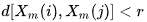
The below figure shows the indicator in two modes (the upper part shows entropy, the lower one features standardized increments):
Fig. 3. Entropy values for the sliding window 50 (above) and fractional differentiation with the degree of 0.8
It can be seen that the values of these two estimates are not correlated, which is a good sign for the machine learning model (absence of multicollinearity) which will be considered in the next section.
On-the-fly Expert Advisor optimization using machine learning: logit regression
Thus we have a suitable differentiated time series which can be used for generating trading signals. It was mentioned above that the time series is more stationary and is more convenient for machine learning models. We also have the series persistence evaluation. Now we need to select an optimal machine learning algorithm. Since the EA must be optimized within itself, there is a requirement for the learning speed, which must be very fast and must have minimal delays. For these reasons I have chosen logistic regression.
Logistic regression is used to predict the probability of an event based on the values of a set of variables x1, x2, x3 ... xN, which are also called predictors or regressors. In our case, the variables are the indicator values. It is also necessary to introduce the dependent variable y which is usually equal to either 0 or 1. Thus, it can serve as a signal to buy or to sell. Based on the values of the regressors, calculate the probability of that the dependent variable belongs to a particular class.
An assumption is made that the probability of occurrence of y = 1 is equal to: ![]() where
where ![]() are the vectors of values of independent variables 1, x1, x2 ... xN and the regression coefficients, respectively, and f(z) is the logistic function, or sigmoid:
are the vectors of values of independent variables 1, x1, x2 ... xN and the regression coefficients, respectively, and f(z) is the logistic function, or sigmoid: 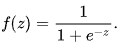 As a result, the y distribution function for the given x can be written as follows:
![]()
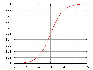
Fig. 4. Logistic curve (sigmoid). Source: Wikipedia.
We will not describe in detail the logistic regression algorithm, because it is widely known. Let us use the ready-made CLogitModel class from the Alglib library.
Creating an Auto Optimizer class
Let us create a separate class CAuto_optimizer which will represent a combination of the simple virtual tester and the logit regression:
//+------------------------------------------------------------------+
//|Auto optimizer class                                              |
//+------------------------------------------------------------------+
class CAuto_optimizer
  {
private:
// Logit regression model |||||||||||||||
   CMatrixDouble     LRPM;
   CLogitModel       Lmodel;
   CLogitModelShell  Lshell;
   CMNLReport        Lrep;
   int               Linfo;
   double            Lout[];
//||||||||||||||||||||||||||||||||||||||||
   int               number_of_samples, relearn_timout, relearnCounter;
   virtual void      virtual_optimizer();
   double            lVector[][2];
   int               hnd, hnd1;

public:
                     CAuto_optimizer(int number_of_sampleS, int relearn_timeouT, double diff_degree, int entropy_window) {
                             this.number_of_samples = number_of_sampleS;
                             this.relearn_timout = relearn_timeouT;
                             relearnCounter = 0;
                             LRPM.Resize(this.number_of_samples, 5);
                             hnd = iCustom(NULL, 0, "fractional entropy", false, diff_degree, 1e-05, number_of_sampleS, entropy_window);
                             hnd1 = iCustom(NULL, 0, "fractional entropy", true, diff_degree, 1e-05, number_of_sampleS, entropy_window);
                            }
                     ~CAuto_optimizer() {};
   double            getTradeSignal();
  };
The following is created in the //Logit regression model// section: a matrix for the x and y values, the logit model Lmodel and its auxiliary classes. After training the model, the Lout[] array will receive the probabilities of the signal belonging to any of the classes, 0:1.
The constructor received the size of the learning window number_of_samples, period after which the model will be re-optimized relearn_timout, and the fractional differentiation degree for the diff_degree indicator, as well as the entropy calculation window entropy_window.
Let us consider in detail the virtual_optimizer() method:
//+------------------------------------------------------------------+
//|Virtual tester                                                    |
//+------------------------------------------------------------------+
CAuto_optimizer::virtual_optimizer(void) {
   double indarr[], indarr2[];
   CopyBuffer(hnd, 0, 1, this.number_of_samples, indarr);
   CopyBuffer(hnd1, 0, 1, this.number_of_samples, indarr2);
   ArraySetAsSeries(indarr, true); ArraySetAsSeries(indarr2, true);

   for(int s=this.number_of_samples-1;s>=0;s--) {
      LRPM[s].Set(0, indarr[s]);
      LRPM[s].Set(1, indarr2[s]);
      LRPM[s].Set(2, s);

      if(iClose(NULL, 0, s) > iClose(NULL, 0, s+1)) {
         LRPM[s].Set(3, 0.0);
         LRPM[s].Set(4, 1.0);
      }
      else {
         LRPM[s].Set(3, 1.0);
         LRPM[s].Set(4, 0.0);
      }
    }

    CLogit::MNLTrainH(LRPM, LRPM.Size(), 3, 2, Linfo, Lmodel, Lrep);

    double profit[], out[], prof[1];
    ArrayResize(profit,1); ArraySetAsSeries(profit, true); profit[0] = 0.0;
    int pos = 0, openpr = 0;

    for(int s=this.number_of_samples-1;s>=0;s--) {
      double in[3];
      in[0] = indarr[s]; in[1] = indarr2[s]; in[2] = s;
      CLogit::MNLProcess(Lmodel, in, out);

      if(out[0] > 0.5 && !pos) {pos = 1; openpr = s;};
      if(out[0] < 0.5 && !pos) {pos = -1; openpr = s;};

      if(out[0] > 0.5 && pos == 1) continue;
      if(out[0] < 0.5 && pos == -1) continue;

      if(out[0] > 0.5 && pos == -1) {
         prof[0] = profit[0] + (iClose(NULL, 0, openpr) - iClose(NULL, 0, s));
         ArrayInsert(profit, prof, 0, 0, 1); pos = 0; }

      if(out[0] < 0.5 && pos == 1) {
         prof[0] = profit[0] + (iClose(NULL, 0, s) - iClose(NULL, 0, openpr));
         ArrayInsert(profit, prof, 0, 0, 1); pos = 0; }
    }
 GraphPlot(profit);
}
The method is obviously very simple and is therefore quick. The first column of the LRPM matrix is filled in a loop with the indicator values + linear trend value (it was added). In the next loop, the current close price is compared to the previous one in order to clarify the probability of a deal: buy or sell. If the current value is greater than the previous one, then there was a buy signal. Otherwise this was a sell signal. Accordingly, the following columns are filled with the values 0 and 1.
Thus this is a very simple tester which is not aimed to optimally select signals but simple reads them at each bar. The tester can be improved by method overloading, which is however beyond the scope of this article.
After that the logit regression is trained using the MNLTrain() method which accepts the matrix, its size, the number of variables x (only one variable is passed here for each case), the Lmodel class object to save the trained model to it and auxiliary classes.
After training, the model is tested and displayed in the optimizer window as a balance chart. This is visually efficient allowing to show how the model was trained on the learning sample. But the performance is not analyzed from the algorithmic point of view.
The virtual optimizer is called from the following method:
//+------------------------------------------------------------------+
//|Get trade signal                                                  |
//+------------------------------------------------------------------+
double CAuto_optimizer::getTradeSignal() {
   if(this.relearnCounter==0)
      this.virtual_optimizer();
   relearnCounter++;
   if(this.relearnCounter>=this.relearn_timout) this.relearnCounter=0;

   double in[], in1[];
   CopyBuffer(hnd, 0, 0, 1, in); CopyBuffer(hnd1, 0, 0, 1, in1);
   double inn[3]; inn[0] = in[0]; inn[1] = in1[0]; inn[2] = relearnCounter + this.number_of_samples - 1;
   CLogit::MNLProcess(Lmodel, inn, Lout);
   return Lout[0];
}
It checks the number of bars which have passed since the last training. If the value exceeds the specified threshold, the model should be re-trained. After that the last value of indicators is copied along the units of time which passed since the last training. This is input into the model using the MNLProcess() method which returns the result showing whether the value belongs to a class 0:1, i.e. the trading signal.
Creating an Expert Advisor to test the library operation
Now we need to connect the library to a trading Expert Advisor and add the signal handler:
#include <MT4Orders.mqh>
#include <Math\Stat\Math.mqh>
#include <Trade\AccountInfo.mqh>
#include <Auto optimizer.mqh>

input int       History_depth = 1000;
input double    FracDiff = 0.5;
input int       Entropy_window = 50;
input int       Recalc_period = 100;
sinput double   MaximumRisk=0.01;
sinput double   CustomLot=0;
input int       Stop_loss = 500;           //Stop loss, positions protection
input int       BreakEven = 300;           //Break even
sinput int      OrderMagic=666;

static datetime last_time=0;

CAuto_optimizer *optimizer = new CAuto_optimizer(History_depth, Recalc_period, FracDiff, Entropy_window);
double sig1;
Expert Advisor settings are simple and include the window size History_depth, i.e. the number of training examples for the auto optimizer. The differentiation degree FracDiff and the number of received bars Recalc_period after which the model will be re-trained. Also the Entropy_window setting has been added for adjusting the entropy calculation window.
The last function receives a signal from a trained model and performs trading operations:
void placeOrders(){
   if(countOrders(0)!=0 || countOrders(1)!=0)   {
      for(int b=OrdersTotal()-1; b>=0; b--)
         if(OrderSelect(b,SELECT_BY_POS)==true) {
          if(OrderType()==0 && sig1 < 0.5) if(OrderClose(OrderTicket(),OrderLots(),OrderClosePrice(),0,Red)) {};
          if(OrderType()==1 && sig1 > 0.5) if(OrderClose(OrderTicket(),OrderLots(),OrderClosePrice(),0,Red)) {};
      }
    }

   if(countOrders(0)!=0 || countOrders(1)!=0) return;
   if(sig1 > 0.5 && (OrderSend(Symbol(),OP_BUY,lotsOptimized(),SymbolInfoDouble(_Symbol,SYMBOL_ASK),0,0,0,NULL,OrderMagic,INT_MIN)>0)) { return; }
   if(sig1 < 0.5 && (OrderSend(Symbol(),OP_SELL,lotsOptimized(),SymbolInfoDouble(_Symbol,SYMBOL_BID),0,0,0,NULL,OrderMagic,INT_MIN)>0)) {}
  }
If the probability of buying is greater than 0.5, then this is a buy signal and/or a signal to close a sell position. And vice-versa.
Testing of the self-optimizing EA and conclusions
Let's proceed to the most interesting part, i8.e. to tests.
The Expert Advisor was run with the specified hyperparameters without genetic optimization, i.e. almost at random, on the EURUSD pair with the 15-minute timeframe, at Open prices.
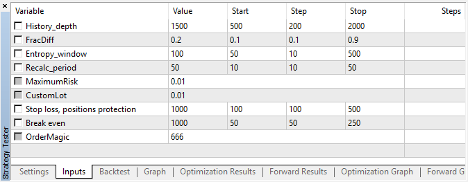
Fig. 5. Tested Expert Advisor settings
Fig. 6. Results of testing with the specified settings
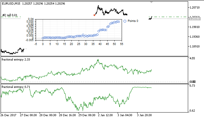
Fig. 7. Virtual tester results in the training sample
In this interval, the implementation showed a stable growth, which means that the approach can be interesting for further analysis.
As a result, we tried to achieve three goals in one article, including the following:
- understanding of the market "memory",
- evaluation of memory in terms of entropy,
- development of self-optimizing Expert Advisors.