Practical application of correlations in trading
Alexander Fedosov | 6 March, 2019
Table of contents
- Introduction
- The concept of correlation
- Types of correlations
- Implementation of indicators
- Correlation-based trading system
- Testing the trading system
- Findings
- Conclusions
Introduction
The essence of trading is connected with the necessity to predict future market developments, and thus the potential profit strongly depends on the accuracy of such prediction. At the beginning of my article Trading ideas based on price direction and movement speed, I described the following idea: every movement is characterized by its direction, acceleration and speed. The same is applicable to the price movement in forex and other markets.
Any movement has certain characteristics which indicate the beginning of the movement, a certain speed, inertia and end. Successful trading strategies are those which can detect the movement beginning as soon as possible and enter the market, as well as clearly identify the end of this movement. Nevertheless, no strategy can determine the entry and exit points with an absolute probability. This is a matter of a favorable chance and probability. Therefore, in this article we will consider one of the probability theory tools — correlation, which will be applied in the framework of financial markets.
The concept of correlation
Correlation is a statistical relationship between two or more random variables (or quantities which can be considered random with some acceptable degree of accuracy). Changes in one ore more variables lead to systematic changes of other related variables. The mathematical measure of the correlation of two random variables is the correlation coefficient. If a change in one random variable does not lead to a regular change in the other random variable but leads to a change in another statistical characteristic of this random variable, such a relation is not considered correlation, although it is statistical.
The correlation coefficient values can vary from -1 to +1. The closer the correlation value to 1, the higher the interdependence between the variables studied. And if the value tends to 1, correlation is considered positive. If the value tends to -1, correlation is negative. During positive correlation, an increase in one of the variables leads to an increase in the second one. In case with the negative correlation, an increase in one value leads to a decrease in the second one.
In other worlds, correlations helps identify the dependence of one variable on the second one based on the available data. How can correlation help in financial market trading?
Let us view Fig.1 and the marked downtrend zone.
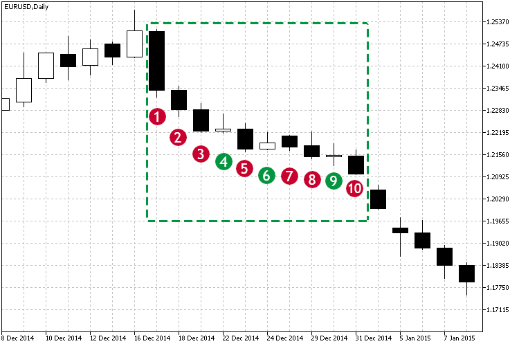
Fig.1 Example of a downtrend.
As can be seen form the marked zone, starting with the candlestick #1, most of the close prices are below the open price, and each close price is below the previous one. Thus, the price is falling. It can be seen visually, that there is a downtrend. But how can you understand whether the dependency us strong? Moreover, the trend is not perfect: there were small attempts to move upwards at candlesticks 4, 6 and 9. How can correlation be helpful here? In this case the correlation coefficient will indicate the strength of the current movement. Based on observations of the correlation coefficients over time, we can make several conclusions:
- The strength of the current trend - directly based on the current value of the correlation.
- The duration of the trend - based on the observation of the selected threshold value over time. For example, threshold is over 0.75 and does not fall within 3-4 candlesticks.
Types of correlations
The following types of correlation help in defining the dependence between the analyzed variables:
- Linear and nonlinear. Linear correlation refers to a dependence, in which one value increases or decreases, and the second one changes accordingly. In nonlinear dependence, changes in one variable do not lead to a direct change in the other one, but can be described by other functions.
- Positive and negative correlation refers to the character of this dependence. In case of positive correlation, growth in one of the variables leads to the growth of the other one.
See Fig.1 which shows an example of linear negative correlation. Next, we consider various types of calculation and methods for determining interdependence of two variables.
Linear correlation coefficient (Pearson correlation coefficient)
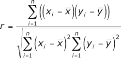
This calculation method allows identifying the direct relationship between variables based on their absolute values. The calculation is organized so that if the relationship between the variables is linear, the Pearson coefficient will show it. In the context of financial markets, this relationship would mean the presence of movement in one or other direction in time. The Pearson correlation is calculated according to the following formula:
Now let us calculate Pearson correlation coefficient for the data presented in Fig.1 and measure the dependence of Close prices over time. To do this, let's enter the data in the table:
| Close price | Candlestick number |
|---|---|
| 1.23406 | 1 |
| 1.22856 | 2 |
| 1.22224 | 3 |
| 1.22285 | 4 |
| 1.21721 | 5 |
| 1.21891 | 6 |
| 1.21773 | 7 |
| 1.21500 | 8 |
| 1.21546 | 9 |
| 1.20995 | 10 |
The entire calculation is shown in the next figure.
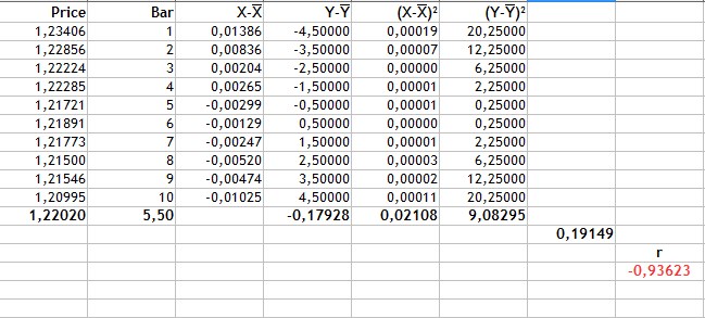
Fig.2 Calculation of Pearson correlation coefficient.
The calculation is performed in the following sequence:
- First, the average values of the Price and of the candlestick number are calculated. These are 1.22020 and 5.5 respectively.
- Then we will find deviation from the mean for each variable type (columns 3-4).
- The value of -0.17928 is the sum of the product of price deviations and the candlestick number. It is the numerator of the formula.
- Columns 5 and 6 are the squared deviations. Values of 0.02108 and 9.08295 are square roots of the sum of squared deviations.
- The denominator in the formula or the product of the sum of squared deviations is equal to 0.19149.
- Then, the Pearson correlation coefficient is equal to -0.93623.
Spearman's rank correlation coefficient
This calculation method enables the determining of a direct linear relationship between random variables. The evaluation is based not on the numerical values of the analyzed elements, but on the corresponding ranks. Its values can also vary from -1 to 1. The absolute value characterizes the closeness of the interconnection, while the sign denotes the direction of this connection between the two elements. It is calculated using the following formula:
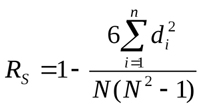
Where Di is the rank difference of the studied characteristics. Let us consider an example of calculating the rank correlation for data presented in Fig.1 and enter the values in the new table:
| Close price | Candlestick number | Close price rank | Candlestick number rank |
|---|---|---|---|
| 1.23406 | 1 | 10 | 1 |
| 1.22856 | 2 | 9 | 2 |
| 1.22224 | 3 | 7 | 3 |
| 1.22285 | 4 | 8 | 4 |
| 1.21721 | 5 | 4 | 5 |
| 1.21891 | 6 | 6 | 6 |
| 1.21773 | 7 | 5 | 7 |
| 1.21500 | 8 | 2 | 8 |
| 1.21546 | 9 | 3 | 9 |
| 1.20995 | 10 | 1 | 10 |
As can be seen from the table, we have ranked the values of the Close price: rank 1 is assigned to the lowest value, and so on. Using the formula, we calculate the difference of D ranks of the characteristics studied and substitute the obtained values into the formula.
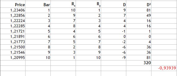
Fig.3 Calculation of the Spearman's rank correlation coefficient.
As can be seen from Fig.3, we find the difference of ranks, then find the sum of the squared resulting differences and get 320. Substitute the obtained values into the formula and get the result of -0.93939.
Based on the resulting value of the correlation coefficient we can get the same conclusion: a strong linear negative relationship. In this case, the closeness of the connection is comparable to the Pearson correlation coefficient. However the following fact should be taken into account: this calculation method has one disadvantage. Incomparable values of differences can correspond to the same values of rank differences. For example, bar ranking is comparable, while the values of price ranks are not even, though the variation of the price is rather small and differs by thousandths. Therefore, this calculated method is appropriate in this case.
Kendall rank correlation coefficient
Like the Spearman's coefficient, Kendall rank correlation coefficient is the measure of linear relationship between random variables. Values of analyzed elements are ranked similarly, though the calculation method is different. The following coefficient calculation formula is applied here:
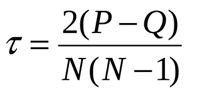
Where P is the sum of matches and Q is the sum of inversions. To understand the meaning of the above, let us once again view the example in Fig.1. Let us first sort the table data as follows:
| Close price | Candlestick number | Close price rank | Candlestick number rank |
|---|---|---|---|
| 1.20995 | 10 | 1 | 10 |
| 1.21500 | 8 | 2 | 8 |
| 1.21546 | 9 | 3 | 9 |
| 1.21721 | 5 | 4 | 5 |
| 1.21773 | 7 | 5 | 7 |
| 1.21891 | 6 | 6 | 6 |
| 1.22224 | 3 | 7 | 3 |
| 1.22285 | 4 | 8 | 4 |
| 1.22856 | 2 | 9 | 2 |
| 1.23406 | 1 | 10 | 1 |
So, the table is sorted by the Close price rank. After that let us determine the number of ranks higher than the current one, starting with the first row in the 'Candlestick number rank' field. The first value is 10, so let's check it - there are no ranks above one. Then view 8 and find a higher rank of 9. And so on. These will be P matching values.
Then we calculate lower ranks. For 10, there will be 9 lower ranks, because it is the highest one. 8 will have seven lower ranks — 5,7,6,3,4,2,1. These will be Q inversions. Let us add the resulting value to a table and calculate the coefficient:
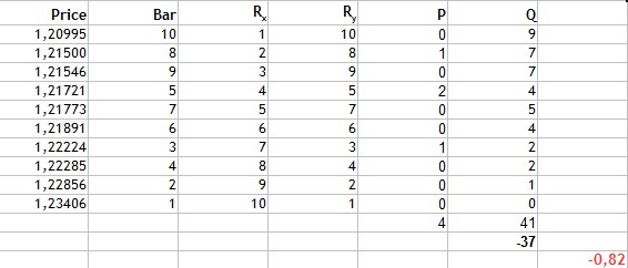
Fig.4 Calculation of Kendall rank correlation coefficient.
Then we sum up the resulting matching values and inversion values. Their difference is equal to -37. By inserting this value into the formula, we get the Kendall coefficient equal to -0,82. It is again a strong negative correlation. However the result suggests that this method is more selective, than the previous two ones, because the absolute value is smaller.
The Fechner signs correlation coefficient
This method is based on the evaluation of the degree of consistency in the directions of value deviations from the mean value and the calculation of the signs of deviations corresponding to the values. The calculation formula is very simple:
Here Na is the number of matches by the sign, Nb is the number of mismatches. Now let us calculate the correlation coefficient for our example from fig.1.
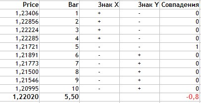
Fig.4 Calculation of Fechner correlation coefficient.
The calculation is performed as follows:
- Average data values for two characteristics are found. This is equal to 1.2202 for the price and 5.5 for the candlestick number.
- In the Sign X column, we set '+' if the current Price value is greater than the average and '-' if Price is below average.
- The same is done for the candlestick number values.
- Then we need to calculate matching signs for the two characteristics (the Price and the candlestick number).
- As can be seen from the table, the values matched only once and thus Na = 1, while Nb = 9.
- These obtained values are substituted in the formula.
As you can see, the Fechner correlation coefficient calculation method is quite simple. The resulting value is -0,8. Again, this is an indication of a strong negative relationship between the Close price and the candlestick number.
Implementation of indicators
Now, let us implement all the correlation calculation methods using the MQL5 language.
Pearson correlation coefficient
Since the Pearson coefficient is calculated using a large formula, the calculation is divided into two stages, calculation of the numerator and the denominator.
//+------------------------------------------------------------------+
//| Calculation of the numerator                                     |
//+------------------------------------------------------------------+
double Numerator(double &Ranks[],int N)
  {
//----
   double Y[],dx[],dy[],mx=0.0,my=0.0,sum=0.0,sm=0.0;
   ArrayResize(Y,N);
   ArrayResize(dx,N);
   ArrayResize(dy,N);

   int n=N;
   for(int i=0; i<N; i++)
     {
      Y[i]=n;
      n--;
     }

   mx=Average(Y);
   my=Average(Ranks);

   for(int j=0;j<N;j++)
     {
      dx[j]=Y[j]-mx;
      dy[j]=Ranks[j]-my;
      sm+=dx[j]*dy[j];
     }
   return sm;
  }
//+------------------------------------------------------------------+
//| Calculation of the denominator                                   |
//+------------------------------------------------------------------+
double Denominator(double &Ranks[],int N)
  {
//----
   double Y[],dx2[],dy2[],mx=0.0,my=0.0,sum=0.0,smx2=0.0,smy2=0.0;
   ArrayResize(Y,N);
   ArrayResize(dx2,N);
   ArrayResize(dy2,N);

   int n=N;
   for(int i=0; i<N; i++)
     {
      Y[i]=n;
      n--;
     }

   mx=Average(Y);
   my=Average(Ranks);

   for(int j=0;j<N;j++)
     {
      dx2[j]=MathPow(Y[j]-mx,2);
      dy2[j]=MathPow(Ranks[j]-my,2);
      smx2+=dx2[j];
      smy2+=dy2[j];
     }
   return(MathSqrt(smx2*smy2));
  }
The final calculation method and calculation logic for indicator visualization look as follows:
//+------------------------------------------------------------------+
//| Custom indicator iteration function                              |
//+------------------------------------------------------------------+
int OnCalculate(const int rates_total,    // number of bars in history at the current tick
                const int prev_calculated,// number of bars calculated at previous call
                const int begin,          // bars reliable counting beginning index
                const double &price[]
                )

  {
   if(rates_total<rangeN+begin)
      return(0);
   int limit;

   if(prev_calculated>rates_total || prev_calculated<=0)
     {
      limit=rates_total-2-rangeN-begin;
      if(begin>0)
         PlotIndexSetInteger(0,PLOT_DRAW_BEGIN,rangeN+begin);
     }
   else
      limit=rates_total-prev_calculated;

   ArraySetAsSeries(price,true);

   for(int i=0; i<=limit; i++)
     {
      for(int k=0; k<rangeN; k++)
         PriceInt[k]=price[k+i];
      ExtLineBuffer[i]=PearsonCalc(PriceInt,rangeN);
     }

   return(rates_total);
  }

//+------------------------------------------------------------------+
//| Calculation of Pearson correlation coefficient                   |
//+------------------------------------------------------------------+
double PearsonCalc(double &Ranks[],int N)
  {
   double ch,zn;
   ch=Numerator(Ranks,N);
   zn=Denominator(Ranks,N);
   return (ch/zn);
  }
Spearman's rank correlation coefficient
For an indicator based on this calculation methods, I used some of the existing solutions available here.
//+------------------------------------------------------------------+
//| Custom indicator iteration function                              |
//+------------------------------------------------------------------+
int OnCalculate(const int rates_total,    // number of bars in history at the current tick
                const int prev_calculated,// number of bars calculated at previous call
                const int begin,          // bars reliable counting beginning index
                const double &price[]
                )

  {
   if(rates_total<rangeN+begin)
      return(0);
   int limit;

   if(prev_calculated>rates_total || prev_calculated<=0)
     {
      limit=rates_total-2-rangeN-begin;
      if(begin>0)
         PlotIndexSetInteger(0,PLOT_DRAW_BEGIN,rangeN+begin);
     }
   else
      limit=rates_total-prev_calculated;

   ArraySetAsSeries(price,true);

   for(int i=limit; i>=0; i--)
     {
      for(int k=0; k<rangeN; k++)
         PriceInt[k]=int(price[i+k]*multiply);

      RankPrices(TrueRanks,PriceInt);
      ExtLineBuffer[i]=SpearmanCalc(R2,rangeN);
     }

   return(rates_total);
  }
//+------------------------------------------------------------------+
//| Calculation of Spearman correlation coefficient                  |
//+------------------------------------------------------------------+
double SpearmanCalc(double &Ranks[],int N)
  {
//----
   double sumd2=0.0;

   for(int i=0; i<N; i++)
      sumd2+=MathPow(Ranks[i]-i-1,2);

   return(1-6*sumd2/(N*(MathPow(N,2)-1)));
  }
Kendall rank correlation coefficient
For the calculation of this method, let is use the internal reserves of MQL5 itself. Namely, we will use the built-in mathematical statistics library.
//+------------------------------------------------------------------+
//| Custom indicator iteration function                              |
//+------------------------------------------------------------------+
int OnCalculate(const int rates_total,    // number of bars in history at the current tick
                const int prev_calculated,// number of bars calculated at previous call
                const int begin,          // bars reliable counting beginning index
                const double &price[]
                )

  {
   if(rates_total<rangeN+begin)
      return(0);
   int limit;

   if(prev_calculated>rates_total || prev_calculated<=0)
     {
      limit=rates_total-2-rangeN-begin;

      if(begin>0)
         PlotIndexSetInteger(0,PLOT_DRAW_BEGIN,rangeN+begin);
     }
   else
      limit=rates_total-prev_calculated;

   ArraySetAsSeries(price,true);

   for(int i=0; i<=limit; i++)
     {
      for(int k=0; k<rangeN; k++)
         PriceInt[k]=price[k+i];
      ExtLineBuffer[i]=KendallCalc(PriceInt,rangeN);
     }

   return(rates_total);
  }
//+------------------------------------------------------------------+
//| Calculation of Kendall correlation coefficient                   |
//+------------------------------------------------------------------+
double KendallCalc(double &Ranks[],int N)
  {
   double Y[],t;
   ArrayResize(Y,N);

   int n=N;
   for(int i=0; i<N; i++)
     {
      Y[i]=n;
      n--;
     }
   MathCorrelationKendall(Ranks,Y,t);
   return (t);
  }
//+------------------------------------------------------------------+
The Fechner signs correlation coefficient
This method is based in the calculation of matching signs of deviations from the average value. Further, matching signs are counted.
//+------------------------------------------------------------------+
//| Custom indicator iteration function                              |
//+------------------------------------------------------------------+
int OnCalculate(const int rates_total,    // number of bars in history at the current tick
                const int prev_calculated,// number of bars calculated at previous call
                const int begin,          // bars reliable counting beginning index
                const double &price[]
                )

  {
   if(rates_total<rangeN+begin)
      return(0);
   int limit;

   if(prev_calculated>rates_total || prev_calculated<=0)
     {
      limit=rates_total-2-rangeN-begin;
      if(begin>0)
         PlotIndexSetInteger(0,PLOT_DRAW_BEGIN,rangeN+begin);
     }
   else
      limit=rates_total-prev_calculated;

   ArraySetAsSeries(price,true);
   for(int i=0; i<=limit; i++)
     {
      for(int k=0; k<rangeN; k++)
         PriceInt[k]=price[k+i];
      ExtLineBuffer[i]=FechnerCalc(PriceInt,rangeN);
     }

   return(rates_total);
  }
//+------------------------------------------------------------------+
//| Calculation of Fechner correlation coefficient                   |
//+------------------------------------------------------------------+
double FechnerCalc(double &Ranks[],int N)
  {
   double Y[],res,mx,my,sum=0.0,markx[],marky[];
   double Na=0.0,Nb=0.0;
   ArrayResize(Y,N);
   ArrayResize(markx,N);
   ArrayResize(marky,N);

   int n=N;
   for(int i=0; i<N; i++)
     {
      Y[i]=n;
      n--;
     }

   mx=Average(Y);
   my=Average(Ranks);

   for(int j=0; j<N; j++)
     {
      markx[j]=(Y[j]>mx)?1:-1;
      marky[j]=(Ranks[j]>my)?1:-1;
      if(markx[j]==marky[j])
         Na++;
      else
         Nb++;
     }

   res=(Na-Nb)/(Na+Nb);
   return (res);
  }
Figure 6 demonstrates all the four methods of calculation of correlation between the candlestick Close price and time. The period of 10 is set for all indicators and thus you can evaluate their operation under similar conditions.
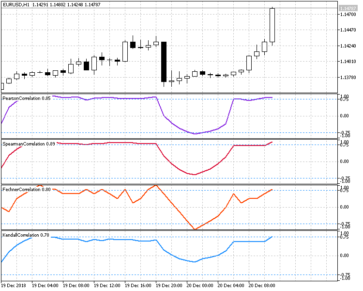
Fig.6 Comparison of different calculation methods.
Correlation-based trading system
When creating a trading strategy based on correlations, you should carefully analyze the indicator specifics and calculation methods as well as identify possible risks and unfavorable market entry conditions.
The use of large periods is not advised for almost all indicators, since the indicator will be lagging. They may also show weak correlations in case of sharp reversals, because they will be accounting for the values of already completed opposite movements.
Since indicators analyze not the current price, but the aggregate of several values over a time period, the current correlation value should not be treated as an absolute estimate. The correlation dynamics should be analyzed. This can be done using oscillators which utilize the current and previous values of the correlation coefficient.
Therefore, our strategy will analyze the behavior of the correlation coefficient based oscillator and will search for a breakout of predefined levels. The following two options are possible:
- The fall of the coefficient. Sell, when the positive coefficient falls and breaks through a predefined key level. Buy, when the negative coefficient grows and breaks through a symmetrical level set in a positive area.
- The growth of the coefficient. Sell, when the coefficient falls in the negative area and breaks through a predefined level. Buy, when the coefficient grows and breaks through a symmetrical positive level.
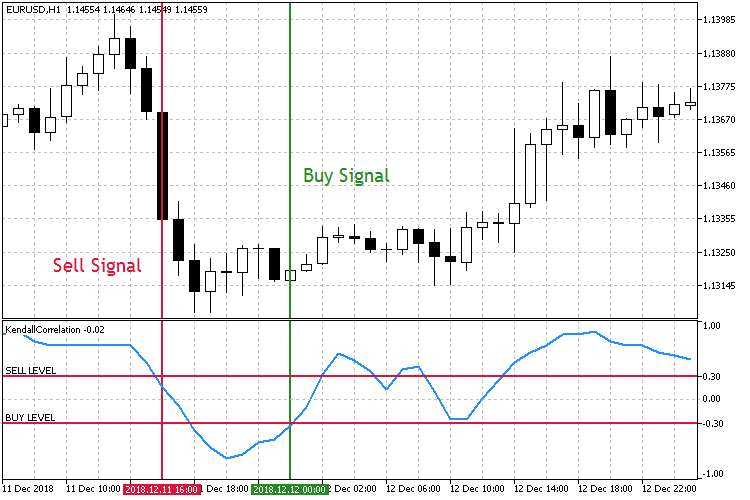
Fig.7 Trading the fall of the correlation coefficient.
As can be seen from the screenshots, there are two symmetrical correlation coefficient levels Sell Level 0.3 and Buy Level -0.3. When the Sell Level is broken downwards, open a Sell order. A Buy order is placed when the Buy Level is broken upwards.
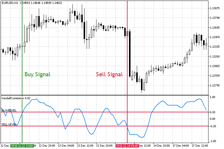
Fig.8 Trading the growth of the correlation coefficient.
In the second trading mode shown in Fig. 8, the key market entry levels are the opposite. This time, when the Buy Level is broken upwards, a buy order is opened. A sell order is opened when the Sell Level is broken downwards.
To implement and Expert Advisor, we need provide the above strategies and choose an appropriate correlation calculation method.
//+------------------------------------------------------------------+
//| Enumeration of operating modes                                   |
//+------------------------------------------------------------------+
enum Strategy_type
  {
   DECREASE = 1,           //On Decrease
   INCREASE                //On Increase
  };
//+------------------------------------------------------------------+
//| Enumeration of correlation calculation methods                   |
//+------------------------------------------------------------------+
enum Corr_method
  {
   PEARSON = 1,            //Pearson
   SPEARMAN,               //Spearman
   KENDALL,                //Kendall
   FECHNER                 //Fechner
  };
In addition to the EA parameters, let us add the following inputs: selection of calculation method, the strategy the key level and the adjustable operating timeframe.
//+------------------------------------------------------------------+
//| Expert Advisor input parameters                                  |
//+------------------------------------------------------------------+
input    string               Inp_EaComment="Correlation Strategy";        //EA Comment
input    double               Inp_Lot=0.01;                                //Lot
input    MarginMode           Inp_MMode=LOT;                               //MM

//--- Выбор метода расчета корреляции и тип стратегии
input    Corr_method          Inp_Corr_method=1;                           //Correlation Method
input    Strategy_type        Inp_Strategy_type=1;                         //Strategy type

//--- EA parameters
input    string               Inp_Str_label="===EA parameters===";         //Label
input    int                  Inp_MagicNum=1111;                           //Magic number
input    int                  Inp_StopLoss=40;                             //Stop Loss(points)
input    int                  Inp_TakeProfit=60;                           //Take Profit(points)
//--- Indicator parameters
input    int                  Inp_RangeN=10;                               //Rang Calculation
input    double               Inp_KeyLevel=0.2;                            //Key Level
input    ENUM_TIMEFRAMES      Inp_Timeframe=PERIOD_CURRENT;                //Working Timeframe
The correctness of the key level will be checked at the EA initialization step: the level must be located between 0 and 1, because an absolute value will be used for the level.
//--- Checking the correctness of the key level
   if(Inp_KeyLevel>1 || Inp_KeyLevel<0)
     {
      Print(Inp_EaComment,": Incorrect key level!");
      return(INIT_FAILED);
     }
Then set the correlation calculation method selected in inputs:
//---
   switch(Inp_Corr_method)
     {
      case 1:
         ind_type="Correlation\\PearsonCorrelation";
         break;
      case 2:
         ind_type="Correlation\\SpearmanCorrelation";
         break;
      case 3:
         ind_type="Correlation\\KendallCorrelation";
         break;
      case 4:
         ind_type="Correlation\\FechnerCorrelation";
         break;
      default:
         break;
     }
//--- Getting the indicator handle
   InpInd_Handle=iCustom(Symbol(),Inp_Timeframe,ind_type,Inp_RangeN);
   if(InpInd_Handle==INVALID_HANDLE)
     {
      Print(Inp_EaComment,": Failed to get indicator handle");
      Print("Handle = ",InpInd_Handle,"  error = ",GetLastError());
      return(INIT_FAILED);
     }
After that, we can set up entry conditions and EA operating logic.
//+------------------------------------------------------------------+
//| Expert tick function                                             |
//+------------------------------------------------------------------+
void OnTick()
  {
//--- Getting data for calculations

   if(!GetIndValue())
      return;

   if(!Trade.IsOpenedByMagic(Inp_MagicNum))
     {
      //--- Opening an order if there is a buy signal
      if(BuySignal())
         Trade.BuyPositionOpen(Symbol(),Inp_Lot,Inp_StopLoss,Inp_TakeProfit,Inp_MagicNum,Inp_EaComment);
      //--- Opening an order if there is a sell signal
      if(SellSignal())
         Trade.SellPositionOpen(Symbol(),Inp_Lot,Inp_StopLoss,Inp_TakeProfit,Inp_MagicNum,Inp_EaComment);
     }
  }
//+------------------------------------------------------------------+
//| Buy conditions                                                   |
//+------------------------------------------------------------------+
bool BuySignal()
  {
   bool res=false;
   if(Inp_Strategy_type==1)
      res=(corr[1]>Inp_KeyLevel && corr[0]<Inp_KeyLevel)?true:false;
   else if(Inp_Strategy_type==2)
      res=(corr[0]>Inp_KeyLevel && corr[1]<Inp_KeyLevel)?true:false;
   return res;
  }
//+------------------------------------------------------------------+
//| Sell conditions                                                  |
//+------------------------------------------------------------------+
bool SellSignal()
  {
   bool res=false;
   if(Inp_Strategy_type==1)
      res=(corr[1]<-Inp_KeyLevel && corr[0]>-Inp_KeyLevel)?true:false;
   else if(Inp_Strategy_type==2)
      res=(corr[0]<-Inp_KeyLevel && corr[1]>-Inp_KeyLevel)?true:false;
   return res;
  }
Testing
The Expert Advisor will be tested with the following parameters:
- Interval: for the Uptrend mode01.01.2015 — 01.12.2018.
- Currency pair: EURUSD.
- Trading mode: No delay. These are not high-frequency trading strategies, so the effect of delays would be very small.
- Testing: M1 OHLC. Pre-testing on real ticks shows nearly the same results.
- Initial deposit: 1000 USD.
- Leverage: 1:500.
- Server: MetaQuotes-Demo.
- Quotes: 5-digit.
Testing and optimization parameters.
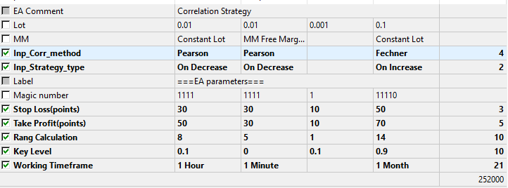
Fig.9 The set of parameters to be optimized.
The optimization will help determine which of the calculation methods and strategy types is more preferable. Testing and optimization produced the following results.
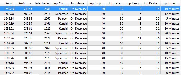
Fog.10 Testing and optimization results.
Now let us test the EA using the best optimization parameters.
Fig.11 Testing results with the best optimization parameters.
Findings
Based on the results obtained, the following observations can be made:
- The best results are obtained with the correlation coefficient fall strategy, in the On Decrease mode. This result can only be explained by the fact that when coefficients fall, the oscillator faster responds to market movements. As mentioned above, oscillators based on correlation coefficients (especially those having large periods) have significant lagging.
- The simplest calculation method (Fechner coefficient) is not found among the top 20 results. The best result with this method is only located in the 99th place.
- The best results were obtained on small timeframes with tight take profit and stop loss.
- No dependencies of profit amount on the selected period and the key level have been found. However smaller periods prevail and the lower limit of the optimization range with the period of 5 is constantly encountered among the best results. This is another confirmation that correlation based indicators have a large delay on large period and show worse results.
Conclusions
The attached archive contains all the listed files, which are located in the appropriate folders. For their proper operation, you only need to save the MQL5 folder into the terminal folder.
Programs used in the article
| # | Name | Type | Declaration |
|---|---|---|---|
| 1 | Correlation.mq5 | EA | The Expert Advisor, which includes 4 correlation calculation methods and 2 strategies based on them. |
| 2 | Trade.mqh | Code Base | A class of trading functions |
| 3 | FechnerCorrelation.mq5 | Indicator | Fechner correlation coefficient calculation indicator |
| 4 | KendallCorrelation.mq5 | Indicator | Kendall correlation coefficient calculation indicator |
| 5 | PearsonCorrelation.mq5 | Indicator | Pearson correlation coefficient calculation indicator |
| 6 | SpearmanCorrelation.mq5 | Indicator | Spearman correlation coefficient calculation indicator |