Practical Use of Kohonen Neural Networks in Algorithmic Trading. Part II. Optimizing and forecasting

In this article, we continue considering Kohonen networks as a trader's tool. In Part I, we corrected and improved the publicly available neural network classes, having added necessary algorithms. Now, it is time to apply them to practice. In this article, we are going to use Kohonen maps in solving problems, such as selecting the optimal EA parameters and forecasting time series.

Searching for the optimal EA parameters

Common Principles

The problem of optimizing robots is solved in many trading platforms, including MetaTrader. The embedded Tester offers a wide variety of tools, advanced algorithms, distributed calculations, and fine-grained statistical evaluations. However, from the user point of view, there is always one more critical last stage in optimization, i.e., the stage of choosing the final working parameters, based on the analysis of that barrage of information generated by the program. In the preceding articles dealing with Kohonen maps and published on this website, examples of visually analyzing the optimization results were provided. However, this suggests that the user performs expert analysis him or herself. Ideally, we would like to get more specific recommendations from the neural network. All in all, algorithmic trading is trading by a program without involving the user.

Upon completing optimization, we usually receive a long tester report with many options. Depending on the column to sort by, we extract from its depths absolutely different settings that mean optimality on a relevant criterion, such as profit, Sharpe ratio, etc. If even we have determined a criterion we trust in most, the system often offers several settings with the same result. How to choose?

Some traders practice their own synthetic criterion that includes several standard indexes into calculations — with this approach, it is really less possible to receive equal strings in the report. However, they, in fact, translate the matter into the area of the meta-optimization of the mentioned criterion (how to choose its formula correctly?). And this is a separate topic. So, we will return to analyzing the standard optimization results.

In my opinion, selecting the optimal set of EA parameters must be based on searching for the longest lasting "plateau" within the area of the values of a target function with the pre-set minimum level of that "plateau", rather than on searching for the maximum of such function. In trading context, the level of the "plateau" can be compared to average profitability, while its length can be compared to reliability, i.e., to the robustness and stability of the system.

After we have purposefully considered some data analysis techniques in Part I, it is suggested that such "plateaus" can be searched for using clusterization.

Unfortunately, there are no unified or universal methods to obtain clusters with the required characteristics. Particularly, if the number of clusters is "too" large, they become small and demonstrate all the symptoms of re-learning — they generalize information poorly. If there are "too" few clusters, then they are rather undertrained, so they receive into themselves the samples that are fundamentally different. The term of "too" does not have any clear definitions, since there is a specific threshold for each task, number, and structure of data. Therefore, it is usually suggested to perform several experiments.

Number of clusters is logically related to the map size and to the applied task. In our case, the former factor works in only one direction, since we have previously decided to set the size by formula (7). Accordingly, knowing this size, we get an upper limit placed for the number of clusters — there can hardly be more of them than the size of one side. On the other hand, based on the applied task, just a pair of clusters would probably suit us: "Good" and "bad" settings. This is the range within which experiments can be performed. All this is only applicable to algorithms based on a clear indication of the number of clusters, such as K-Means. Our alternative algorithm does not have such a setting, however, due to arranging the clusters by quality, we can just exclude all clusters with numbers above the given one from our consideration.

Then we will try to perform clusterization using Kohonen network. However, we have to discuss a finer point, before we go to practice.

Many robots are optimized across the very large-scale space of parameters. therefore, optimization is performed by a genetic algorithm. It saves time and resources. However, it has a special feature of "falling" into profitable areas. In principle, this was the intention. However, in terms of Kohonen maps, it is not very good. The matter is that Kohonen maps are sensitive to data distribution in the input space and actually reflect it in the resulting topology. Since the bad versions of parameters are excluded by genetics at earlier stages, they occur much rarer than the good ones that are inherited by genetics in very many details. As a result, the Kohonen network may omit to notice the dangerous valleys of the target function near the allegedly good versions found. Since the market characteristics always fluctuate, it is critical to avoid such parameters, at which a left or right step leads to losses.

These are the ways to solve the problem:

1. To give up genetic optimization in favor of the full one; since it is not always possible to the full extent, it is allowed to implement the hierarchic approach, i.e., to perform genetic optimization with a large step first, localize interesting areas, and then perform the full optimization in them (and then analyze using Kohonen network); it is also thought that the overextension of the list of parameters to be optimized provides the system with the number of degrees of freedom, due to which it becomes, first, instable; and second, optimization translates into fitting; therefore, it is recommended to select permanent values for the larger part of parameters, based on their physical meaning and on fundamental analysis (for example, timeframes should be selected according to the strategy type: A day for the intraday strategies, a week for medium-term ones, etc.); then it is possible to reduce the optimization space and abandon genetics;
2. To repeat genetic optimization several times, using as a criterion both maximums and minimums, and zeros of the target function; for example, you can perform optimization triply:
   • By profit factor (PF), as usual;
   • By its inverse quantity, 1/PF;
   • By formula (min(PF, 1/PF) / max(PF, 1/PF)) that would collect statistics around 1;
   After that, to consolidate the results of all optimizations and analyze them by the network as a unified whole;
3. It is a half-measure that is still worth researching: To construct Kohonen maps in a metric excluding the optimized index (actually, all the economic indexes that are not the EA parameters); in other words, in teaching the network, the measure of similarity between the neuron weights and inputs must only be calculated by the selected components relevant to the EA parameters; reverse metric is interesting, too, where the proximity measures are only calculated by economic indexes, and we probably see the topological dispersion in the planes of parameters, which provides evidence of the instability of the system; in both cases, the weights of neurons are fitted in a complete manner — by all components.

Last version N3 means that the network topology will only reflect the distribution of the EA parameters (or economic indexes, depending on the direction). Indeed, when we teach the network on the full rows from the optimization table, the columns, such as profit, drawdown, and number of deals, form the total distribution of neurons to the extent no less than that of the EA parameters. This may be good for the visual analysis problem to reach a general understanding and draw the conclusions of which parameters affect mostly which indexes. But this is bad for analyzing our parameters, since their real distribution is altered by economic indexes.

In principle, for the case of analyzing the optimization results, there is obvious dividing the input vector into two logically separate components: The EA inputs and its indexes (output). Teaching a Kohonen network on a full vector, we are trying to identify the dependence of "inputs" and "outputs" (a two-directional unconditional relationship). When the network is only taught on a part of features, we can try and see the directed relationships: How "outputs" are clustered depending on "inputs" or, vice versa, how "inputs" are clustered depending on "outputs." We will consider both options.

Further development of SOM-Explorer

To implement this teaching mode with masking some features, some further development of classes CSOM and CSOMNode will be required.

Distances are calculated in class CSOMNode. Excluding specific components from calculations is unified for all objects of the class, so we will make the relevant variables statistic:

    static int dimensionMax;
    static ulong dimensionBitMask;

dimensionMax allows setting the maximum amount of the neuron weights to be calculated. For example, if the space dimensionality is 5, then the dimensionMax equal to 4 shall mean that the last component of the vector is excluded from calculations.

dimensionBitMask allows excluding the randomly arranged components using a bit mask: If the ith bit equals to 1, then the ith component is processed; if it equals to 0, then it is not.

Let us add the static method to place the variables:

static void CSOMNode::SetFeatureMask(const int dim = 0, const ulong bitmask = 0)
{
  dimensionMax = dim;
  dimensionBitMask = bitmask;
}

Now, we are going to change the distance calculations using new variables:

double CSOMNode::CalculateDistance(const double &vector[]) const
{
  double distSqr = 0;
  if(dimensionMax <= 0 || dimensionMax > m_dimension) dimensionMax = m_dimension;
  for(int i = 0; i < dimensionMax; i++)
  {
    if(dimensionBitMask == 0 || ((dimensionBitMask & (1 << i)) != 0))
    {
      distSqr += (vector[i] - m_weights[i]) * (vector[i] - m_weights[i]);
    }
  }
  return distSqr;
}

Now, we only have to make sure that class CSOM puts limitations in neurons in a proper manner. Let us add a similar public method to CSOM:

void CSOM::SetFeatureMask(const int dim, const ulong bitmask)
{
  m_featureMask = 0;
  m_featureMaskSize = 0;
  if(bitmask != 0)
  {
    m_featureMask = bitmask;
    Print("Feature mask enabled:");
    for(int i = 0; i < m_dimension; i++)
    {
      if((bitmask & (1 << i)) != 0)
      {
        m_featureMaskSize++;
        Print(m_titles[i]);
      }
    }
  }
  CSOMNode::SetFeatureMask(dim == 0 ? m_dimension : dim, bitmask);
}

In the test EA, we will create string parameter FeatureMask, in which the user may set a feature mask, and parse it for the availability of symbols '1' and '0':

    ulong mask = 0;
    if(FeatureMask != "")
    {
      int n = MathMin(StringLen(FeatureMask), 64);
      for(int i = 0; i < n; i++)
      {
        mask |= (StringGetCharacter(FeatureMask, i) == '1' ? 1 : 0) << i;
      }
    }
    KohonenMap.SetFeatureMask(0, mask);

All this is done immediately before launching the Train method and, therefore, affects the calculations of distances both during learning and at the stage of calculating U-Matrix and clusters. However, in some cases, it will be interesting to us to perform clusterization by other rules, such as teaching the network without any mask and applying the mask to find clusters only. For this purpose, we will additionally introduce control parameter ApplyFeatureMaskAfterTraining equal to 'false' by default. however, if it is set to 'true', we will call SetFeatureMask after Train.

While we are at improving our tools yet again, we will cover one more point relating to the fact that we are going to use the working settings of trading robots as input vectors.

It would be convenient to upload the values of the EA parameters to the network to analyze them directly from the set-file. For this purpose, we write the following function:

bool LoadSettings(const string filename, double &v[])
{
  int h = FileOpen(filename, FILE_READ | FILE_TXT);
  if(h == INVALID_HANDLE)
  {
    Print("FileOpen error ", filename, " : ",GetLastError());
    return false;
  }
  
  int n = KohonenMap.GetFeatureCount();
  ArrayResize(v, n);
  ArrayInitialize(v, EMPTY_VALUE);
  int count = 0;

  while(!FileIsEnding(h))
  {
    string line = FileReadString(h);
    if(StringFind(line, ";") == 0) continue;
    string name2value[];
    if(StringSplit(line, '=', name2value) != 2) continue;
    int index = KohonenMap.FindFeature(name2value[0]);
    if(index != -1)
    {
      string values[];
      if(StringSplit(name2value[1], '|', values) > 0)
      {
        v[index] = StringToDouble(values[0]);
        count++;
      }
    }
  }
  
  Print("Settings loaded: ", filename, "; features found: ", count);
  
  ulong mask = 0;
  for(int i = 0; i < n; i++)
  {
    if(v[i] != EMPTY_VALUE)
    {
      mask |= (1 << i);
    }
    else
    {
      v[i] = 0;
    }
  }
  if(mask != 0)
  {
    KohonenMap.SetFeatureMask(0, mask);
  }
 
  FileClose(h);
  return count > 0;
}

In it, we parse the set-file strings and find in them the names of parameters, which correspond with the features of a taught network. The coinciding settings are saved in the vector, while the non-coinciding ones are skipped. The feature mask is filled with unities only for the available components. The function returns the logical feature of the fact that the settings have been read.

Now, when we have this function at our disposal, to download the parameters from the files of settings, we will insert the following strings into the branch of the if-operator where there is checking of DataFileName != "":

      // process .set file as a special case of pattern
      if(StringFind(DataFileName, ".set") == StringLen(DataFileName) - 4)
      {
        double v[];
        if(LoadSettings(DataFileName, v))
        {
          KohonenMap.AddPattern(v, "SETTINGS");
          ArrayPrint(v);
          double y[];
          CSOMNode *node = KohonenMap.GetBestMatchingFeatures(v, y);
          Print("Matched Node Output (", node.GetX(), ",", node.GetY(),
            "); Hits:", node.GetHitsCount(), "; Error:", node.GetMSE(),
            "; Cluster N", node.GetCluster(), ":");
          ArrayPrint(y);
          KohonenMap.CalculateOutput(v, true);
          hasOneTestPattern = true;
        }
      }

The settings will be marked with SETTINGS.

Working EA

Now, we are inching closer to the problem of selecting the optimal parameters.

To test the theories of clustering the optimization results, first of all, we have to create a working EA. I have generated it using MQL5 Wizard and some standard modules and named it WizardTest (its source code is attached in the end of this article). Here is the list of inputs:

input string             Expert_Title                 ="WizardTest"; // Document name
ulong                    Expert_MagicNumber           =17897;        // 
bool                     Expert_EveryTick             =false;        // 
//--- inputs for main signal
input int                Signal_ThresholdOpen         =10;           // Signal threshold value to open [0...100]
input int                Signal_ThresholdClose        =10;           // Signal threshold value to close [0...100]
input double             Signal_PriceLevel            =0.0;          // Price level to execute a deal
input double             Signal_StopLevel             =50.0;         // Stop Loss level (in points)
input double             Signal_TakeLevel             =50.0;         // Take Profit level (in points)
input int                Signal_Expiration            =4;            // Expiration of pending orders (in bars)
input int                Signal_RSI_PeriodRSI         =8;            // Relative Strength Index(8,...) Period of calculation
input ENUM_APPLIED_PRICE Signal_RSI_Applied           =PRICE_CLOSE;  // Relative Strength Index(8,...) Prices series
input double             Signal_RSI_Weight            =1.0;          // Relative Strength Index(8,...) Weight [0...1.0]
input int                Signal_Envelopes_PeriodMA    =45;           // Envelopes(45,0,MODE_SMA,...) Period of averaging
input int                Signal_Envelopes_Shift       =0;            // Envelopes(45,0,MODE_SMA,...) Time shift
input ENUM_MA_METHOD     Signal_Envelopes_Method      =MODE_SMA;     // Envelopes(45,0,MODE_SMA,...) Method of averaging
input ENUM_APPLIED_PRICE Signal_Envelopes_Applied     =PRICE_CLOSE;  // Envelopes(45,0,MODE_SMA,...) Prices series
input double             Signal_Envelopes_Deviation   =0.15;         // Envelopes(45,0,MODE_SMA,...) Deviation
input double             Signal_Envelopes_Weight      =1.0;          // Envelopes(45,0,MODE_SMA,...) Weight [0...1.0]
input double             Signal_AO_Weight             =1.0;          // Awesome Oscillator Weight [0...1.0]
//--- inputs for trailing
input double             Trailing_ParabolicSAR_Step   =0.02;         // Speed increment
input double             Trailing_ParabolicSAR_Maximum=0.2;          // Maximum rate
//--- inputs for money
input double             Money_FixRisk_Percent=5.0;          // Risk percentage

For the purpose of our studies, we are going to optimize just a few parameters, not all of them.

Signal_ThresholdOpen
Signal_ThresholdClose
Signal_RSI_PeriodRSI
Signal_Envelopes_PeriodMA
Signal_Envelopes_Deviation
Trailing_ParabolicSAR_Step
Trailing_ParabolicSAR_Maximum

I performed the genetic optimization of the EA from January to June, 2018 (20180101-20180701) on EURUSD D1, M1 OHLC, by profit. the set-file with the settings of parameters to be optimized is attached in the end of this article (WizardTest-1.set). Optimization results were saved to file Wizard2018plus.csv (attached in the end hereof, too), from which outliers are excluded, particularly those with the amount of deals below 5 and with the sky-high, irreal Sharpe factors. Moreover, since the genetic optimization produced, by definition, a shift to profitable passages, I decided to completely exclude the losing ones and only kept the entries where the profit had made at least 10,000.

I also removed a pair of index columns, since they are actually dependent on other ones, such as balance or Expected Payoff, and there are some other candidates, such as PF (Profit Factor), RF (Rally Factor), and Sharpe factor — highly intercorrelated, plus, RF is inversely correlated with drawdown, but I have kept them in place to demonstrate this dependence on the maps.

Selecting the structure of inputs with the minimum set of independent components that could bear the maximum of information is a critical condition for efficiently using neural networks.

Having opened the csv-file containing the optimization results, we will see that questionable matter I have mentioned above: A huge amount of strings containing equally profitable indexes and different parameters. Let us try and exercise a reasonable option.

To have a reference point for evaluating our selected option in future, let us look at the forward test for the set of parameters from the very first string of the optimization results (see WizardTest-1.set). Test dates are July 1, 2018 to December 1, 2018.

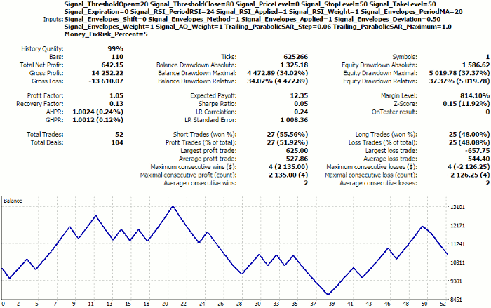
Tester report on the first listed selection of settings

Remember these, actually, not very good figures, we are going to take to the network.

Neural network analysis

Number of entries in the csv-file is about 2,000. Therefore, the Kohonen network size calculated by formula (7) will be 15.

We launch CSOM-Explorer, enter the data file name (Wizard2018plus.csv) in DataFileName, 15 — in CellsX and CellsY, and keep EpochNumber equal to 100. To view all the planes simultaneously, we select small images: 210 for each of ImageW and ImageH and 6 for MaxPictures. As a result of the EA operation, we will substantially obtain as follows:

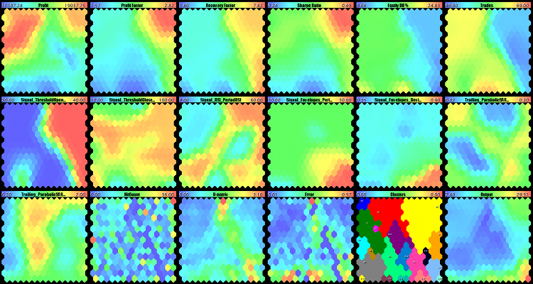
Teaching the Kohonen network on the EA optimization results

The upper row fully consists of the maps of economic indexes, the second row and the first map of the third row are the EA's working parameters, and, finally, the last 5 maps are special maps constructed in Part I.

Let us have a closer look at the maps:

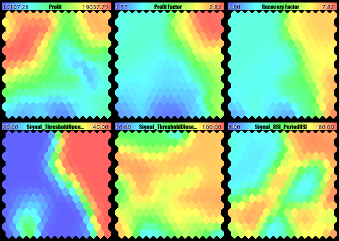
Profit, PF, RF, and the first three parameters of the working EA

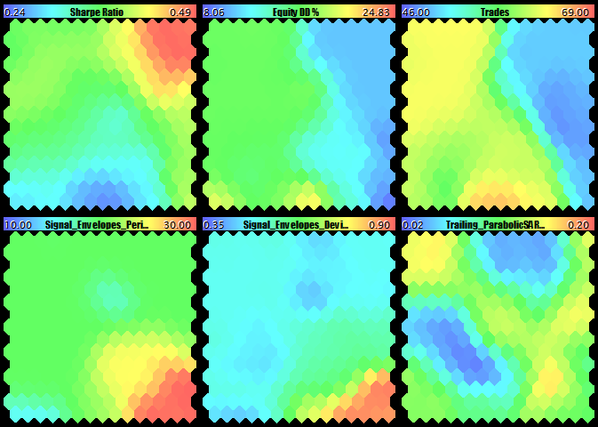
Sharpe factor, drawdown, number of trades, and the second three parameters of the EA

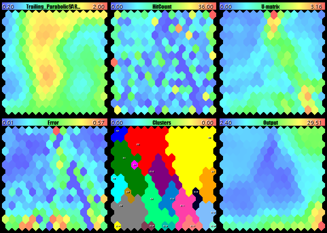
The last parameter of the EA, as well as the counter of hits, U-Matrix, quantization errors, clusters, and the network output

Let us perform the expert analysis of the obtained maps, as it were, manually.

In terms of profits, we can see two suitable areas with the approximately equal values (in red) in the top-right and top-left corner, the right one being larger and highlighted more intensively. However, the parallel analysis of the planes with PF, RF, and Sharpe factor convinces us of the top-right corner being the best choice. This is also confirmed by the less drawdown.

Let us go to components that are relevant to the EA parameters, paying attention to the top-right corner. In the maps of the first five parameters, this spot is stably colored, which allows us to confidently name the optimal values (point with the mouse cursor at the upper right neuron in each map to see the relevant value in the tip):

Signal_ThresholdOpen = 40
Signal_ThresholdClose = 85
Signal_RSI_PeriodRSI = 73
Signal_Envelopes_PeriodMA = 20
Signal_Envelopes_Deviation = 0.5

the maps of the two remaining parameters change their color actively in the top-right corner, so it is unclear which values to choose. Judging by the plane with the counter of hits, the top-rightest neuron is preferable. It is also reasonable to make sure that it is a "quiet atmosphere" for it on U-Matrix and on the errors map. Since everything is ok there, we select these values:

Trailing_ParabolicSAR_Step = 0.15
Trailing_ParabolicSAR_Maximum = 1.59

Let us run the EA with those parameters (see WizardTest-plus-allfeatures-manual.set) on the same forward period till December 1, 2018. We will obtain the following result.

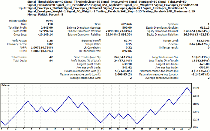
Tester report on the settings selected based on visually analyzing Kohonen maps

The result is remarkably better than that selected randomly from the first string. However, it can still disappoint professionals, so it is worth making a remark here.

This is a test EA, not a grail. Its task is to generate source data to demonstrate how neural network-based algorithms work. After the article has been published, it will become possible to test the tools on a large amount of real trading systems and, perhaps, adapt them for a better usage.

Let us compare the current result to the man values that could be obtained for all the options of settings from csv-files within the same range of dates.

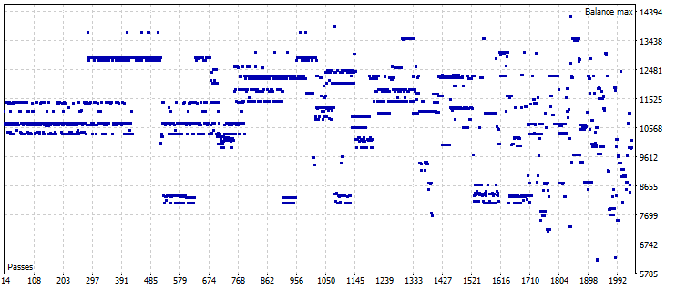
Results of all forward tests

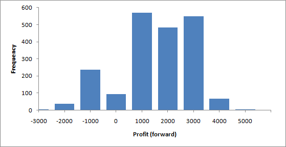
Profit distribution statistics in forward testing

Statistics are as follows: Mean is 1,007, standard deviation is 1,444, median is 1,085, and the lowest and the highest values are -3,813.78 and 4,202.82, respectively. Thus, using expert evaluation, we have obtained the profit even higher than the mean plus standard deviation.

Our task is to learn how to make the same or qualitatively similar choice automatically. To do so, we will use clusterization. Since clusters are numbered in the order of their preferable use, we will consider cluster 0 (though, basically, clusters 1-5 can be used for trading with a portfolio of settings).

Colors of the clusters on the map are always related to their indexing numbers as listed below:

{clrRed, clrGreen, clrBlue, clrYellow, clrMagenta, clrCyan, clrGray, clrOrange, clrSpringGreen, clrDarkGoldenrod}

This may help identify them on smaller images where it is difficult to distinguish the numbers.

SOM-Explorer displays in the log the coordinates of cluster centers, for example, for the current map:

Clusters [20]:
[ 0] "Profit"                        "Profit Factor"                 "Recovery Factor"               "Sharpe Ratio"                 
[ 4] "Equity DD %"                   "Trades"                        "Signal_ThresholdOpen"          "Signal_ThresholdClose"        
[ 8] "Signal_RSI_PeriodRSI"          "Signal_Envelopes_PeriodMA"     "Signal_Envelopes_Deviation"    "Trailing_ParabolicSAR_Step"   
[12] "Trailing_ParabolicSAR_Maximum"
N0 [3,2]
[0] 18780.87080     1.97233     3.60269     0.38653    16.76746    63.02193    20.00378
[7]    65.71576    24.30473    19.97783     0.50024     0.13956     1.46210
N1 [1,4]
[0] 18781.57537     1.97208     3.59908     0.38703    16.74359    62.91901    20.03835
[7]    89.61035    24.59381    19.99999     0.50006     0.12201     0.73983
...

In the beginning, there is the legend of features. Then, for each cluster, there is its number, X and Y coordinates, and the values of features.

Here, for the 0th cluster, we have the following working EA's parameters:

Signal_ThresholdOpen=20
Signal_ThresholdClose=66
Signal_RSI_PeriodRSI=24
Signal_Envelopes_PeriodMA=20
Signal_Envelopes_Deviation=0.5
Trailing_ParabolicSAR_Step=0.14
Trailing_ParabolicSAR_Maximum=1.46

We will run a forward test with these parameters (WizardTest-plus-allfeatures-auto-nomasks.set) and receive the report:

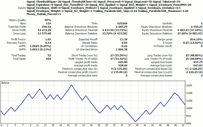
Tester report for the settings selected automatically from the clusters of Kohonen maps without the feature mask

The result is not much better than the first random test, and it is remarkably worse than the expert one. It's all about clusterization quality. At the moment, it is being performed by all the features at once, including both economic indexes and the EA parameters. However, we should search for the "plateau", in terms of trading figures only. Let us apply to clusterization the feature mask that considers only them, i.e., the first six ones. To do so, set:

FeatureMask=1111110000000
FeatureMaskAfterTraining=true

And then restart learning. Clusterization in SOM-Explorer is performed as the final learning stage, and the clusters obtained are saved in the network file. This is necessary for the network loaded later to be immediately used for "recognizing" new samples. Such samples may contain fewer than all the indexes (i.e., the vector may be incomplete), such as with analyzing the set-files — it only contains the EA's parameters, but there are no economic indexes (and they have no sense). Therefore, for such samples, their own feature mask is constructed in function LoadSettings, which mask corresponds with the existing components of the vector, and then that mask is applied to the network. Thus, the clusterization mask must be implicitly present in the network in order not to conflict with the mask of the vector to be "recognized."

But let us get back to learning using the new mask. It will change the plane of U-Matrix and of clusters. The pattern of clusters will change significantly (left image is before applying the mask, while the right one is after applying the mask).

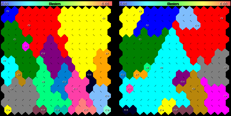
Clusters on Kohonen maps constructed without (left) and with (right) applying the mask by economic indexes

Now, the values of the zero cluster are different.

N0 [14,1] 
[0] 17806.57263     2.79534     6.78011     0.48506    10.70147    49.90295    40.00000
[7]    85.62392    73.51490    20.00000     0.49750     0.13273     1.29078

If you remember, we selected in our expert evaluation the neuron located in the top-right corner, i.e., that having coordinates [14,0]. Now, the system offers us the neighboring neuron [14,1]. Their weights are not very different. Let us move the settings proposed to the working EA's parameters.

Signal_ThresholdOpen=40
Signal_ThresholdClose=86
Signal_RSI_PeriodRSI=74
Signal_Envelopes_PeriodMA=20
Signal_Envelopes_Deviation=0.5
Trailing_ParabolicSAR_Step=0.13
Trailing_ParabolicSAR_Maximum=1.29

We will obtain the following results:

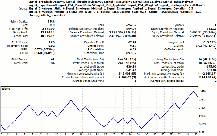
Tester report for the settings selected automatically from the clusters of Kohonen maps, using the mask of economic indexes

They are identical to expert results, regardless of some differences in parameters.

To facilitate moving the clusterization results to the EA settings, we will write a helper function that will generate the set-file with the names and values of the features of the selected cluster (zero, by default). The function is named SaveSettings and gets in the operation if new parameter SaveClusterAsSettings contains the index of the cluster to be exported. By default, this parameter contains -1, which means that there is no need to generate the set-file. It is clear that this function does not "know" about the applied sense of the features and saves them all named in the set-file, so trading indexes, such as Profit, Profit Factor, etc., will be there, as well. User can copy from the generated file only features that correspond with the real parameters of the EA. The values of the parameters are saved as real numbers, so they will have to be corrected for the integer-type parameters.

Now that we are able to save the found settings in portable form, let us create settings for cluster 0 (Wizard2018plusCluster0.set) and load them back to SOM-Explorer (it should be reminded that our utility has already been able to read set-files). In parameter NetFileName, it is necessary to specify the name of the network created at the previous learning stage (it must be Wizard2018plus.som, since we used the data of Wizard2018plus.csv — upon each learning cycle, it is saved in the file, the name of which is that of the input one, but with the extension of .som). In parameter DataFileName, we will specify the name of the set-file generated. Mark SETTINGS will be overlapped with the center of cluster C0.

We will rename the som-file with the network, for it not to be re-written during the subsequent experiments.

The first experiment will be as follows. We will teach the network with a "reverse" mask — by the EA parameters, having excluded trading figures. To do so, we will specify again file Wizard2018plus.csv in parameter DataFileName, clear parameter NetFileName, and set 

FeatureMask=0000001111111

Please note that FeatureMaskAfterTraining is still set to 'true', that is the mask affects clusterization only.

Upon completion of learning, we will load the taught network and test out set-file on it. To do so, we will move the name of the created network file Wizard2018plus.som to parameter NetFileName and copy Wizard2018plusCluster0.set to DataFileName again. The total set of maps will remain unchanged, while U-Matrix and, therefore, the clusters will become different.

The clusterization result is shown in the image below, at the left:

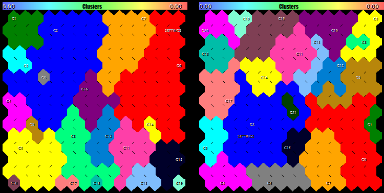
Clusters on Kohonen maps constructed with a mask on the EA parameters: Only at clusterization stage (at the left) and at the network learning and clusterization stage (at the right)

The selection of settings is confirmed by the fact that they get to the zero cluster and that it is larger in size.

As the second experiment, we will teach the network once again with the same mask (by the EA parameters). However, we will extend it on the learning phase, too:

FeatureMaskAfterTraining=false

The full set of maps is shown below, while the changes in clusters are shown to a larger scale in the image above, at the right. Here, neurons are clustered up by the similarity of parameters only. These maps should be read as follows: What economic indexes are expected to appear at the selected parameters? Although the testing settings fell in cluster number 2 (it is worse than 2, but not much), its size is one of the largest ones, which is a positive feature.

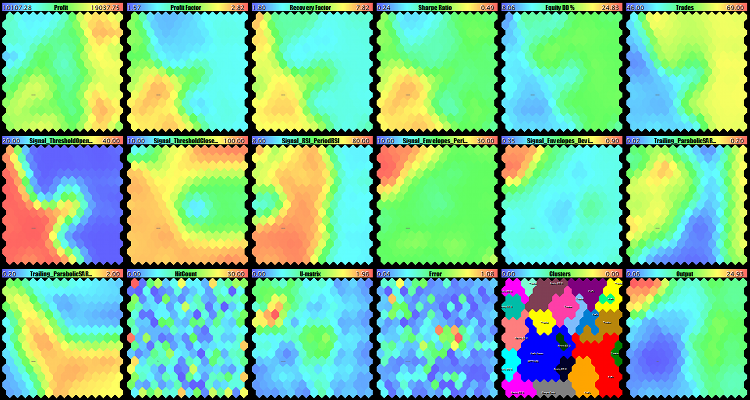
Kohonen maps constructed with a mask by the EA parameters

An interested reader will notice that the maps with economic indexes are not of such an expressed topological nature anymore. However, it is not necessary now, since the essence of checking is identifying the structure of clusters based on the parameters and making sure that the selected settings are well located in this system of clusters.

An "inversed" research would be the full learning and clusterization with the mask by economic indexes:

FeatureMask=1111110000000
FeatureMaskAfterTraining=false

This is the result:

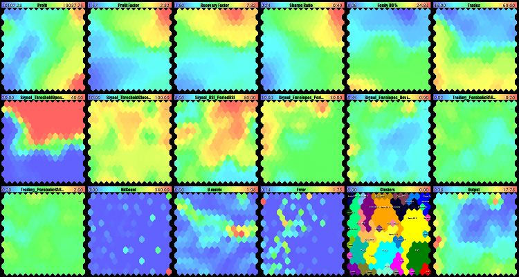
Kohonen maps constructed with a mask by economic indexes

Now, contrast colors are concentrated in the first six planes of economic indexes, while the maps of parameters are rather amorphous. Particularly, we can see that the values of parameters Trailing_ParabolicSAR_Step and Trailing_ParabolicSAR_Maximum do not practically change (the maps are monotonic), it means that they can be excluded from optimization, having based on something average, such as 0.11 and 1.14, respectively. Among the map of parameters, Signal_ThresholdOpen stands out with its contrast, and it becomes clear from it that it is necessary to choose Signal_ThresholdOpen equal to 0.4 to trade successfully. Map U-Matrix is obviously divided into two "pools", the upper and the lower ones, where the upper one is for success and the lower one for failure. Map of hits is very scarce and non-uniform (the largest part of the space is gaps, while active neurons have a large value of the counter), since profits are grouped by several obvious levels in the EA under research.

These maps should be read as follows: What parameters are expected to appear at the selected economic indexes?

Finally, for the last experiment, we will slightly develop SOM-Explorer for it to be able to name clusters reasonably. Let us write function SetClusterLabels that will analyze the values of the specific components of code vectors inside each cluster and compare them to the value range of those components. As soon as the weight value in a neuron approaches to the highest or lowest value, this will be the reason for marking it with the name of the relevant component. For example, if the weight of the 0th relationship (corresponding with profit) exceeds the weights in other clusters, it means that this cluster is characterized by high profit. It should be noted that the sign of the extremum, maximum or minimum, is determined by the meaning of the indication: For profit, the higher the value is, the better; for drawdown, it is vice versa. In this connection, we introduce a special input, FeatureDirection, in which we are going to mark the indications with positive effect with the sign of '+' and those with the negative effect with the sign of '-', while those that are not important or have no sense will be skipped using the sign of ','. Note that, in our case, it would be reasonable to mark only economic indexes, since the values of the EA's working parameters can be whatsoever and are not interpreted as good or bad depending on their proximity to the boundaries of the range of definitions. Therefore, let us set the value of FeatureDirection for the first six features only:

FeatureDirection=++++-+

This is how the labels look for the network with learning on the full vector and clusterization by economic indexes (at the left) and for the network with learning and clusterization with a mask on the EA parameters.

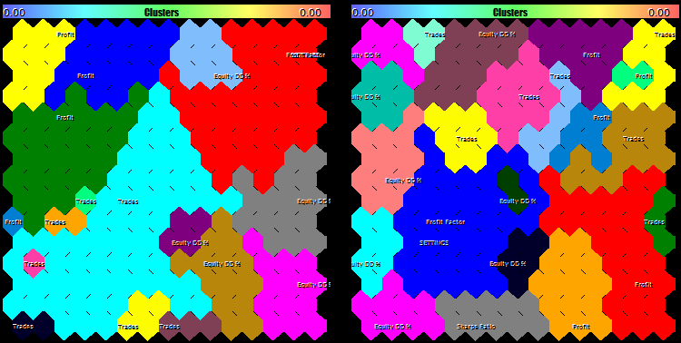
Cluster labels given the cases of: Using a mask by economic indexes at the clusterization stage (at the left) and using a mask by parameters at the learning and clusterization stages (at the right)

We can see that, in both cases, the settings selected fall in the clusters of Profit Factor, so we can expect the highest efficiency in this indication. However, it should be taken into consideration that we have all labels positive here, since the source data is obtained from genetic optimization that acts as a filter for selecting acceptable options. If the data of the full optimization is analyzed, then we can identify clusters that are negative by their nature.

Thus, we have considered in general terms the search for EA's optimal parameters using clusterization on Kohonen maps. As this approach is flexible, so it is complicated. It implies using various clusterization and network teaching methods, as well as preprocessing the inputs. Search for optimal options also depends very much on the specificity of the working robot. The tool presented, SOM-Explorer, allows us to start studying up this slice of data processing, as well as expand and improve it.

Colored classification of the optimization results

Since clusterization methods and quality strongly affect the correct search for the EA's optimal settings, let us try and solve the same problem by a simpler method without evaluating the proximity of neurons.

Let us display the weights of features on a Kohonen map within the RGB color model and select the palest point. Since the RGB color model consists of three planes, we can visualize exactly 3 features in this manner. If there are more or less of them, then we will show the brightness in gray gradations, instead of RGB colors, but still find the palest point.

It should be reminded that, in selecting the features, it is desirable to choose the most independent ones (which has already been mentioned earlier herein).

In implementing the new approach, we will simultaneously demonstrate the possibility to expand classes CSOM with our own ones. Let us create class CSOMDisplayRGB, in which we just override some virtual methods of parent class CSOMDisplay and achieve through this that the RGB-map will be displayed instead of the last DIM_OUTPUT plane.

class CSOMDisplayRGB: public CSOMDisplay
{
  protected:
    int indexRGB[];
    bool enabled;
    bool showrgb;

    void CalculateRGB(const int ind, const int count, double &sum, int &col) const;
  
  public:
    void EnableRGB(const int &vector[]);
    void DisableRGB() { enabled = false; };
    virtual void RenderOutput() override;
    virtual string GetNodeAsString(const int node_index, const int plane) const override;
    virtual void Reset() override;
};

the complete code is attached hereto.

To use this version, let us create a modification of SOM-Explorer-RGB and make the following changes.

Add an input to enable the RGB mode:

input bool ShowRGBOutput = false;

The map object will become the derived class:

CSOMDisplayRGB KohonenMap;

We are going to implement the direct display of the RGB plane in a separate code branch:

  if(ShowRGBOutput && StringLen(FeatureDirection) > 0)
  {
    int rgbmask[];
    ArrayResize(rgbmask, StringLen(FeatureDirection));
    for(int i = 0; i < StringLen(FeatureDirection); i++)
    {
      rgbmask[i] = -(StringGetCharacter(FeatureDirection, i) - ',');
    }
    KohonenMap.EnableRGB(rgbmask);
    KohonenMap.RenderOutput();
    KohonenMap.DisableRGB();
  }

It uses parameter FeatureDirection already familiar to us. Using it, we will be able to choose the specific features (of the entire set of features) to be included into the RGB space. For instance, for our example with Wizard2018plus, it is sufficient to write:

FeatureDirection=++,,-

for the first two features, profit and PF, to get into the map directly (they correspond with the signs of '+'), while the fifth feature, drawdown, is an inverted value (it corresponds with the sign of '-'). Features corresponding with ',' are skipped. All the subsequent ones are not considered either. File WizardTest-rgb.set with settings is attached hereto (network file Wizard2018plus.som is supposed to have been available since the previous stage).

This is how the RGB space appears for those settings (at the left).

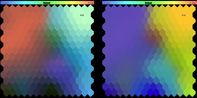
RGB space for features (profit, PF, and drawdown) and (PF, drawdown, and deals)

The colors are relevant to the features in priority sequence: Profit is red, PF is green, and drawdown is blue. The brightest neuron is marked with 'RGB'.

In the log are displayed the coordinates of the 'palest" neuron and the values of its features that can act as an option of the best settings.

Since profit and PF are strongly correlated, we will replace the mask with another one:

FeatureDirection=,+,,-+

In this case, profit is skipped, but the number of deals is added (some brokers offer bonuses for volumes). the result is in the image above (at the right). Here, the color match is different: PF is red, drawdown is green, and number of deals is blue.

If we select only features PF and drawdown, we will obtain a map in gray scale (at the left):

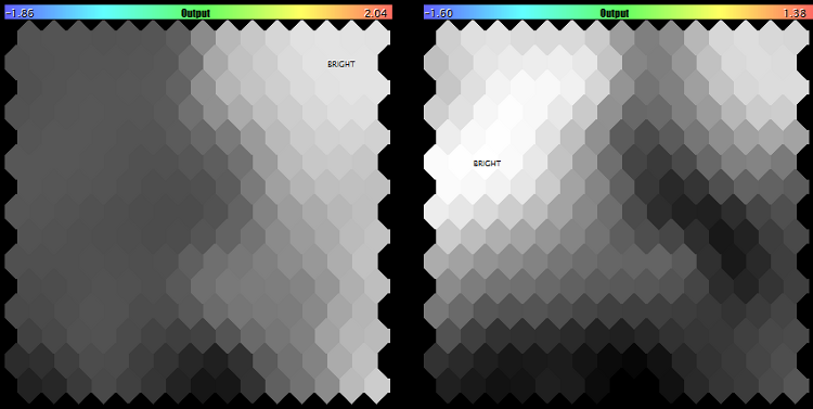
RGB space for features (PF and drawdown) and (profit)

for checking, we can select only one feature, such as profit, and make sure that the black-and-white mode corresponds with the first plane (see above, at the right).

Analysis of forward tests

MetaTrader Tester is known to allow complementing the EA optimization with forward tests on the selected settings. It would be foolish not to try using this information for analysis using Kohonen maps and select the specific option for settings in this manner. Conceptually, clusters or colored areas at the cross-section of high profits in the past and in the future must include settings that provide the most stable income.

To do so, let us take the optimization results of WizardTest together with forward tests (I should remind you that optimization was performed for the profits within the interval of 20180101-20180701, while forward testing was, accordingly, performed on 20180701-20181201), remove all indications from it, except for the profits in the past and in the future, and obtain the new input file for the network — Wizard2018-with-forward.csv (attached hereto). File with settings, WizardTest-with-forward.set, is attached, too.

Teaching the network by all features, including the EA parameters, provides the following result:

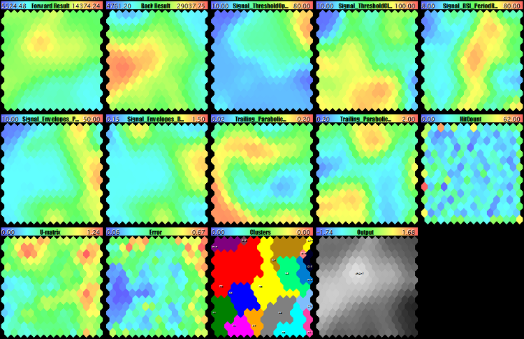
Kohonen maps with forward-test analysis by all features, i.e., profitability factors and the EA parameters

We can see that the area with the future profit is significantly smaller than that of the past profit, and the zero cluster (red) contains this location. Moreover, I included the color analysis by the mask of two indications (FeatureDirection=++), and the palest point on the last map also gets into this cluster. However, neither the cluster center nor the pale point contain any super-profitable settings — although the Tester results are positive, they are two times worse than those obtained earlier.

Let us try to construct a Kohonen map using the mask on the first two features, since only those are indications. To do so, let us apply the other settings with FeatureMask=110000000 (see WizardTest-with-forward-mask11.set) and reteach the network. The result is as follows.

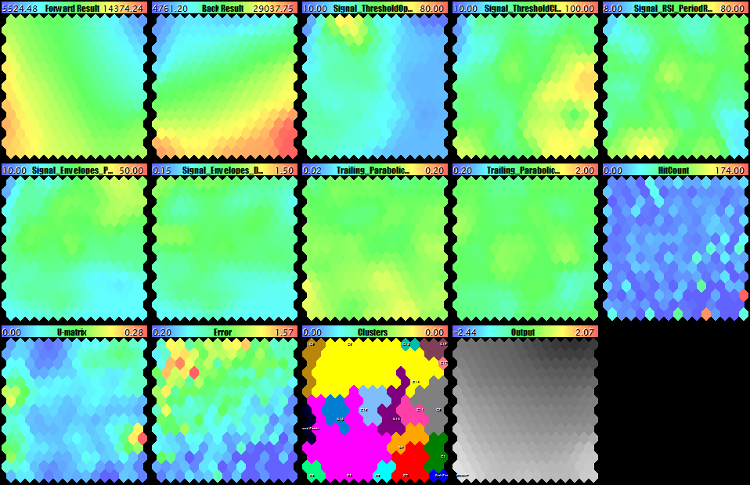
Kohonen maps with forward test analysis by profit factors

Here we can see that the first two planes have got the best expressed spatial structure and crossed the areas with high values (profits) in the bottom left corner that is also highlighted in the last map. Having taken the settings from that neuron, we will obtain the following result:

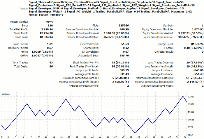
Tester report for the settings selected based on the "profit stability" principle

This, again, is worse than the profit obtained earlier.

Thus, this practical experiment has not allowed us to find optimal settings. At the same time, including the forward testing results into the neural network analysis seems to be correct and should probably become an approach to be recommended. What exactly nuances were lacking to succeed and whether the success is guaranteed in all cases, we propose to discuss in the comments hereto. Perhaps, the result obtained just testifies that our test EA does not suit for stable trading.

Time series forecasting

Overview

Kohonen networks are most frequently used to perform the visual analysis and clusterization of data. However, they can also be used in forecasting. This problem implies that the input data vector represents tic marks, and that its main part normally sized (n - 1), n being the vector size, should be used to forecast the end, which is usually the latest tic mark. Essentially, this problem is similar to that of restituting the noise or partly lost data. However, it has its own specificity.

There are different approaches to forecasting using Kohonen networks. Here are just a few of them.

One Kohonen network (A) learns on the data with incomplete vectors sized (n - 1), i.e., without the last component. For each neuron i of the first network, an additional Kohonen map (Bi) is taught for a truncated set of full vectors sized n, which correspond with those incomplete ones that have been displayed in that neuron i of network A. Based on neurons in network Bi, the probability of the specific values of the last coordinate n is calculated. Later, at the operation stage, the future tick mark is simulated according to the probabilities obtained from network Bi, as soon as the vector to be forecasted gets into neuron i of network A.

Another option. On Kohonen map A is taught on full vectors. The second Kohonen map (B) is taught on modified vectors, in which increments are taken instead of the values, i.e.,

yk = xk+1 - xk, k = 1 .. n - 1

where yk and xk are the components of the initial vector and the modified vector, respectively. Obviously, the size of the modified vector is smaller than that of the initial one by 1. Then, feeding the input of both networks with the teaching data, we calculate the number of the simultaneous displays of the full vector to neuron i in the first network and to neuron j in the second one. Thus, we obtain the conditional probabilities pij of vector y getting into neuron j (in network B), provided that vector x relevant to it has got into neuron i (in network A). At the operation stage, network A is fed with incomplete vector x- (without the last component), the nearest neuron i* by (n - 1) components is found, and then the potential increment is generated according to probabilities pi*. This method, like some other ones, is related to the Monte Carlo method that is about generating random values for the component to be forecasted and finding the most likely outcome according to the statistics of populating the neurons with the data from the teaching selection.

This list can go on much longer, since it includes both the so-called parametrized SOMs and autoregressive models on the SOM neurons, and even the clusterization of stochastic attractors within the space of embedding.

However, all of them are more or less based on the vectors quantization phenomenon that characterizes Kohonen networks. As the network is taught, the weights of neurons asymptotically tend to the mean values of the classes (subsets of inputs) they represent. Each of these mean values provide the best evaluation of the lacking (or future, in case of forecasting) values in the new data with the same statistical law as that in the teaching selection. The more compact and the better divided the classes are, the more precise the evaluation is.

We are going to use the simplest forecasting method based on vectors quantization, which involves the single instance of Kohonen network. However, even this one presents some difficulties.

We will feed the network input with the full vectors of a time series. However, the distances will only be calculated for the first (n - 1) components. Weights will be adapted in full and for all components. Then, for the purpose of forecasting, we will feed the network input with the incomplete vector, find the best neuron for component (n - 1), and read the weight value of the last nth synapse. This will be the forecast.

We have everything ready for this in class CSOM. There is method SetFeatureMask there, which sets the mask on the dimensions of the space of features involved in calculating the distances. However, before implementing the algorithm, we should decide on what exactly we are going to forecast.

Cluster indicator Unity

Among traders, series of quotes are recognized to represent a non-trivial time process. It contains much randomicity, frequent phase changes, and a huge number of influencing factors, and this is, in principle, an open system.

To simplify the problem, we will select for analysis one of the larger timeframes, the daily one. On that timeframe, the noise provides lesser influence than on smaller timeframes. Besides, we will select for forecasting the instrument(s), on which the strong fundamental news that can move the market incalculably appear relatively rarely. In my opinion, the best ones are metals, i.e., gold and silver. Not being a payment instrument of any specific countries and acting both as a raw material and a protective asset, they are less volatile, on the one hand, and they are inextricably connected with currencies, on the other hand.

Theoretically, their future movements should consider the current quotes and respond to Forex quotes.

Thus, we need a way to receive synchronous changes in the prices of metals and basic currencies, represented in the aggregate. At any specific time, this must be a vector with n components, each of which corresponds with the relative cost of a currency or of a metal. And the goal of forecasting consists in forecasting by such a vector the next value of one of the components.

For this purpose, original cluster indicator Unity was created (its source code is attached hereto). The essence of its operation is described with the following algorithm. Let us consider it exemplified as simply as possible, i.e., by one currency pair, EURUSD, and gold, XAUUSD.

Each tic mark (current prices as of the beginning/end of the day) is described by obvious formulas:

EUR / USD = EURUSD

XAU / USD = XAUUSD

where variables EUR, USD, and XAU are certain independent "costs" of assets, while EURUSD and XAUUSD are constants (the known quotes).

To find the variables, let us add one more equation to the system, having limited the sum of squares of the variables by a unity:

EUR*EUR + USD*USD + XAU*XAU = 1

Hence the name of the indicator, Unity.

Using simple substitution, we obtain:

EURUSD*USD*EURUSD*USD + USD*USD + XAUUSD*USD*XAUUSD*USD = 1

From where, we find USD:

USD = sqrt(1 / (1 + EURUSD*EURUSD + XAUUSD*XAUUSD))

and then all other variables.

Or, more generally represented:

x0 = sqrt(1 / (1 + sum(C(xi, x0)**2))), i = 1..n

xi = C(xi, x0) * x0, i = 1..n

where n is the number of variables, C(xi,x0) is the quote of the ith pair that includes the relevant variables. Note that the number of variables is by 1 higher than that of the instruments.

Since coefficients C involved in calculations are quotes that usually deeply vary; in the indicator, they are additionally multiplied by the contract size: Thus, values are obtained that are more or less comparable (or, at least, they are of the same magnitude). To see them in the indicator window (just for one's information), there is an input named AbsoluteValues that should be set to true. By default, it is, of course, equal to false, and the indicator always calculates the increments of the variables:

yi = xi0 / xi1 - 1,

where xi0 and xi1 are values on the last and second last bars, respectively.

We are not going to consider the technical specifics of the indicator implementation here — you can study its source code independently.

Thus, we obtain the following results:

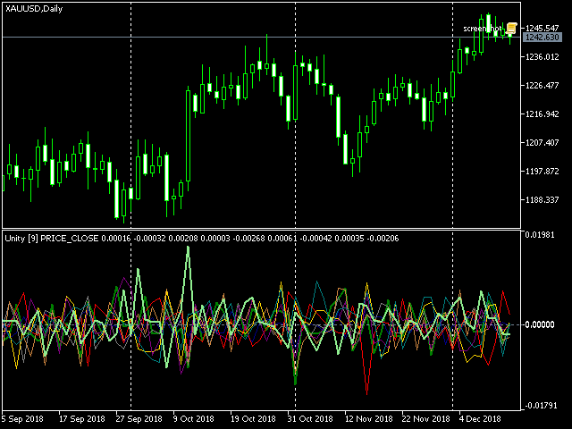
Cluster (multicurrency) indicator Unity, XAUUSD

The lines of the assets composing the working instrument of the current chart (in this case, XAU and USD) are displayed wide, while other lines are of normal thickness.

The following should be mentioned among other inputs of the indicator:

• Instruments — a string with the comma-separated names of working instruments; it is necessary that either base or quote currencies of all instruments are the same;
• BarLimit — number of bars for calculations; as soon as we make it to teaching the neural network, this will become the size of the teaching selection;
• SaveToFile — name of csv-file, to which the indicator exports the values to be subsequently loaded to the neural network; the file structure is simple: The first column is date, all the subsequent ones are the values of the relevant indicator buffers;
• ShiftLastBuffer - flag of switching the mode, in which the csv-file is generated; where the option is false, the data of the same bar are displayed in each string in the file, the number of columns is equal to the number of instruments plus one due to dividing the tickers into components and plus one more column, the very first, for the date; names of the columns correspond with currencies and metals; where the option is true, then an additional column named FORECAST is added, to which the values from the column with the last asset are saved shifted one day forward; thus, in each string, we see both all data of the current day and the tomorrow's change in the last instrument.

For example, to prepare a file with the data to forecast changes in the gold price, you should specify in parameter Instruments: "EURUSD,GBPUSD,USDCHF,USDJPY,AUDUSD,USDCAD,NZDUSD,XAUUSD" (it is important to specify XAUUSD as the last), while 'true' must be specified in ShiftLastBuffer. We will obtain a csv-file with substantially the following structure:

           datetime;      EUR;     USD;      GBP;      CHF;      JPY;      AUD;      CAD;      NZD;      XAU; FORECAST
2016.12.20 00:00:00; 0.001825;0.000447;-0.000373; 0.000676;-0.004644; 0.003858; 0.004793; 0.000118;-0.004105; 0.000105
2016.12.21 00:00:00; 0.000228;0.003705;-0.001081; 0.002079; 0.002790;-0.002885;-0.003052;-0.002577; 0.000105;-0.000854
2016.12.22 00:00:00; 0.002147;0.003368;-0.003467; 0.003427; 0.002403;-0.000677;-0.002715; 0.002757;-0.000854; 0.004919
2016.12.23 00:00:00; 0.000317;0.003624;-0.002207; 0.000600; 0.002929;-0.007931;-0.003225;-0.003350; 0.004919; 0.004579
2016.12.27 00:00:00;-0.000245;0.000472;-0.001075;-0.001237;-0.003225;-0.000592;-0.005290;-0.000883; 0.004579; 0.003232

Please note that the last 2 columns contain the same numbers with a shift by one row. Thus, in the string dated December 20, 2016 we can see both the increment of XAU over that day and its increment over December 21, in column FORECAST.

SOM-Forecast

It is time to implement the forecasting engine, based on Kohonen network. First of all, to understand how it works, we will base on the SOM-Explorer already known and adapt it to the forecasting problem.

The changes center around inputs. Let us remove all everything related to setting the masks: FeatureMask, ApplyFeatureMaskAfterTraining, and FeatureDirection, since the mask for forecasting is known - if the vector sized n tic marks is available, only the first (n - 1) ones should be involved in calculating the distance. But we are going to add a special logical option, ForecastMode, that would allow us to disable this mask, where necessary, and use the classically represented analytical capabilities of Kohonen network. We will need this to explore the market, or rather the system of the instruments specified in Unity, in static state, that is to see correlations within the same day.

In the case of ForecastMode being equal to 'true', we place the mask. If it is 'false', there is no mask.

    if(ForecastMode)
    {
      KohonenMap.SetFeatureMask(KohonenMap.GetFeatureCount() - 1, 0);
    }

As soon as the network has already been taught and the csv-file with test data has been specified in input DataFileName, then we will check the forecasting quality in the ForecastMode as follows:

      if(ForecastMode)
      {
        int m = KohonenMap.GetFeatureCount();
        KohonenMap.SetFeatureMask(m - 1, 0);
        
        int n = KohonenMap.GetDataCount();
        double vector[];
        double forecast[];
        double future;
        int correct = 0;
        double error = 0;
        double variance = 0;
        for(int i = 0; i < n; i++)
        {
          KohonenMap.GetPattern(i, vector);
          future = vector[m - 1]; // preserve future
          vector[m - 1] = 0;      // make future unknown for the net (it's not used anyway due to the mask)
          KohonenMap.GetBestMatchingFeatures(vector, forecast);
          
          if(future * forecast[m - 1] > 0) // check if the directions match
          {
            correct++;
          }
          
          error += (future - forecast[m - 1]) * (future - forecast[m - 1]);
          variance += future * future;
        }
        Print("Correct forecasts: ", correct, " out of ", n, " => ", DoubleToString(correct * 100.0 / n, 2), "%, error => ", error / variance);
      }

Here, each testing vector is presented to the network using GetBestMatchingFeatures, and the response is the 'forecast' vector. Its last component is compared to the correct value from the testing vector. Matching directions are counted in the 'correct' variable, the total forecasting 'error' is accumulated, as related to the scatter of the data itself.

In case of the validation set (parameter ValidationSetPercent is filled) being specified for learning and ReframeNumber being above zero, the new CSOM class function, TrainAndReframe, is involved into operation. It allows us to increase the network size in a staged manner and, tracking the changes in the learning error on the validation set, to stop this process as soon as the error discontinues falling and starts growing. This is the moment where adapting the weights to specific vectors, due to enhancing the computational capabilities of the network, leads to it losing its capability of generalize and work with unknown data.

Having selected the size, we reset ValidationSetPercent and ReframeNumber to 0 and teach the network, as usual, applying the Train method.

Finally, we will slightly change the function of marking in clusters SetClusterLabels. Since assets will be the features and each of them can demonstrate both the positive and the negative extremum, we will include the movement sign into the label. Thus, one and the same feature can be found on the map twice, both with plus and with minus.

void SetClusterLabels()
{
  const int nclusters = KohonenMap.GetClusterCount();

  double min, max, best;
  
  double bests[][3]; // [][0 - value; 1 - feature index; 2 - direction]
  ArrayResize(bests, nclusters);
  ArrayInitialize(bests, 0);
  
  int n = KohonenMap.GetFeatureCount();
  for(int i = 0; i < n; i++)
  {
    int direction = 0;
    KohonenMap.GetFeatureBounds(i, min, max);
    if(max - min > 0)
    {
      best = 0;
      double center[];
      for(int j = nclusters - 1; j >= 0; j--)
      {
        KohonenMap.GetCluster(j, center);
        double value = MathMin(MathMax((center[i] - min) / (max - min), 0), 1);
        
        if(value > 0.5)
        {
          direction = +1;
        }
        else
        {
          direction = -1;
          value = 1 - value;
        }
        
        if(value > bests[j][0])
        {
          bests[j][0] = value;
          bests[j][1] = i;
          bests[j][2] = direction;
        }
      }
    }
  }

  // ...
  
  for(int j = 0; j < nclusters; j++)
  {
    if(bests[j][0] > 0)
    {
      KohonenMap.SetLabel(j, (bests[j][2] > 0 ? "+" : "-") + KohonenMap.GetFeatureTitle((int)bests[j][1]));
    }
  }
}

So, let us consider SOM-Forecast to be ready. We will now try to feed the value input of indicator Unity with it.

Analysis

First, let us try to analyze the entire market (the set of the assets selected) in static, or rather in statistical context, i. e., on the data exported by indicator Unity strictly by days — each string corresponds with the indications on one D1 bar, without any additional column from the 'future'.

For this purpose, we will specify in the indicator the set of Forex instruments, gold, and silver, and the file name in SaveToFile, while we set ShiftLastBuffer to 'false'. An exemplary file, unity500-noshift.csv, obtained in this manner is attached at the end of this article.

Having taught the network on this data using SOM-Forecast (see som-forecast-unity500-noshift.set), we will obtain the following map:

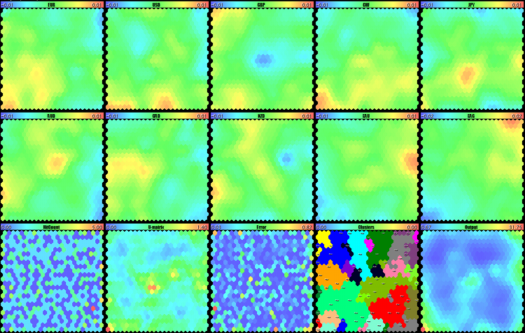
Visual analysis of the Forex market, gold, and silver on Kohonen maps by indicator Unity for D1

Two upper rows are the maps of assets. Comparing them allows us to identify the permanent links that have been working for at least the last 500 days. Particularly, two multicolor spots in the centers catch the eye: It is blue for GBP and yellow for AUD. This means that these assets often were in the reverse phase, and this only refers to strong movements, i.e., the GBPAUD sales prevailed at the breakthrough of the market average variance level. This trend may persist and provides an option for placing pending orders in this direction.

XAG growth is observed in the top right corner, while CHF falls there. And it is vice versa in the bottom left corner: CHF grows, and XAG falls. These assets always diverge at strong movements, so we can trade them by breakthrough in both directions. As expected, EUR and CHF are similar.

Some other specific features can be found on the maps. In fact, even before we started to forecast, we had got a chance to see ahead to some extent.

Let us have a closer look at clusters.

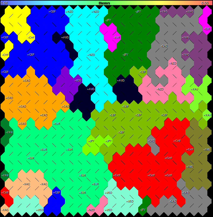
Forex, gold, and silver clusters on Kohonen maps by indicator Unity for D1

They also provide some information, for example, about what usually does not happen (or is seldom the case), namely: EUR does not grow with JPY or CAD falling. GBP often grows simultaneously with CHF falling, and vice versa.

Judging by cluster sizes, currencies EUR, GBP, and CHF are most volatile, i. e., their movements more frequently supersede the movements of other currencies), while USD surprisingly loses out, in this respect, to both JPY and CAD (to be reminded, we calculate changes as %). If we assume that clusters numbers are important, too (we have our clusters sorted), then the first three ones, i. e., +CHF, -JPY, and +GBP, apparently describe the most frequent daily movements (not trend, but exactly the frequency is meant, since even during 'flat' period a larger number of 'steps' upwards may be compensated by one large 'step' downwards).

Now, we will finally go to the forecasting problem.

Forecasting

Let us specify the set of instruments, including Forex and gold ("EURUSD,GBPUSD,USDCHF,USDJPY,AUDUSD,USDCAD,NZDUSD,XAUUSD") in the indicator, number of bars in BarLimit (500 by default), file name in SaveToFile (such as unity500xau.csv), and set flag ShiftLastBuffer to 'true' (mode of creating an additional column for forecasting). Since it is a multicurrency indicator, the number of available data is limited to the shortest history from all instruments. At the server of MetaQuotes-Demo, there is an entirely sufficient number of bars, at least 2,000 bars, for timeframe D1. So, here, it would be helpful to consider another point: Whether it is reasonable to teach the network to such a depth, since the market has most likely changed considerably. 2-3-year history or even 1 year (250 bars on D1) would probably be more suitable for identifying the current regularities.

A sample unity500xau.csv file is attached in the end hereof.

To load it into SOM-Forecast, we will set the following inputs: DataFileName — unity500xau, ForecastMode — true, ValidationSetPercent — 10, and, which is important: ReframeNumber — 10. In this manner, we will both run teaching the network sized 10*10 (default values) and enable checking the error on a validation selection and continuing to teach it with gradually increasing the network size, while the error reduces. Up to 10 increases in size will take place in the TrainAndReframe method, 2 neurons in each dimension. Thus, we will detect the optimal network size for inputs. File with settings (som-forecast-unity500xau.set) is attached.

While gradually teaching and increasing the network, substantially the following is displayed in the log (provided in an abridged form):

FileOpen OK: unity500xau.csv
HEADER: (11) datetime;EUR;USD;GBP;CHF;JPY;AUD;CAD;NZD;XAU;FORECAST
Training 10*10 hex net starts
...
Exit by validation error at iteration 104; NMSE[old]=0.4987230270708455, NMSE[new]=0.5021707785446128, set=50
Training stopped by MSE at pass 104, NMSE=0.384537545433749
Training 12*12 hex net starts
...
Exit by validation error at iteration 108; NMSE[old]=0.4094350709134669, NMSE[new]=0.4238670029035179, set=50
Training stopped by MSE at pass 108, NMSE=0.3293719049246978
...
Training 24*24 hex net starts
...
Exit by validation error at iteration 119; NMSE[old]=0.3155973731785412, NMSE[new]=0.3177587737459486, set=50
Training stopped by MSE at pass 119, NMSE=0.1491464262340352
Training 26*26 hex net starts
...
Exit by validation error at iteration 108; NMSE[old]=0.3142964426509741, NMSE[new]=0.3156342534501801, set=50
Training stopped by MSE at pass 108, NMSE=0.1669971604289485
Exit map size increments due to increased MSE
...
Map file unity500xau.som saved

Thus, the process stopped at the network sized 26*26. Seemingly, we should select 24*24 where the error was the lowest. But really, when working with neural networks, we always play with chances. If you remember, one of parameters, RandomSeed, was responsible for initializing the random data generator used for setting initial weights in the network. Every time changing RandomSeed, we will get a new network with new characteristics. And, all other factors being equal, it will learn better or worse than other instances. Therefore, to select the network size, as well as other settings, including the size of the teaching selection, we usually have to do many trials and make many errors. Then we will follow this principle to decrease the teaching data selection and reduce the network size down to 15*15. Moreover, I sometimes use the non-canonical modification of the described method of the temporal quantization of vectors. the modification consists in teaching the network with flag ForecastMode being disabled and in enabling it when forecasting only. In some cases, this produces a positive effect. Working with neural network never suggests ready-to-eat meals, just recipes. And experiments are not prohibited.

Before teaching, the source file (in our case, unity500xau.csv) should be divided into 2 ones. The matter is that, upon teaching, we will need to verify the forecasting quality on some data. It does not make any sense to do it on the same data that is used by the network for learning (to be more exact, it makes sense just to see it for yourself that the percentage of correct answers is unreally high - you can check this). Therefore, let us copy 50 vectors to test them in a separate file, while teaching the new network using the resting ones. You can find attached the relevant files, unity500xau-training.csv and unity500xau-validation.csv.

Let us specify unity500xau-training in parameter DataFileName (extension .csv is implied), the values of CellsX and CellsY should be 24 each, ValidationSetPercent is 0, ReframeNumber is 0, and ForecastMode is still 'true' (see som-forecast-unity500xau-training.set). As a result of training, we will get the map as follows:

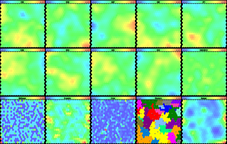
Kohonen network to forecast the movements of gold on D1

This is not forecasting yet, but a visual confirmation that the network has learnt something. What exactly, we will check having fed the input with our validation file.

To do so, let us enter the following settings. File name unity500xau-training will now be transferred to parameter NetFileName (this is the name of the file for the network already taught, which file has the implied extension of .som). In parameter DataFileName, we specify unity500xau-validation. The network will forecast for all the vectors and display statistics in the log:

Map file unity500xau-training.som loaded
FileOpen OK: unity500xau-validation.csv
HEADER: (11) datetime;EUR;USD;GBP;CHF;JPY;AUD;CAD;NZD;XAU;FORECAST
Correct forecasts: 24 out of 50 => 48.00%, error => 1.02152123166208

Alas, the forecast precision is at the level of randomly guessing. Could a grail result from such a simple choice of inputs? Unlikely. Moreover, we chose the history depth at a guess, while this matter must be investigated, too. We should also play with the set of instruments, such as add silver, and, in general, clarify, which of the assets depends more on the other ones, to facilitate the forecasting. Below we will consider an example using silver.

To introduce more context in the inputs, I added into indicator Unity the option of forming a vector based both on just one day and on several last ones. For this purpose, parameter BarLookback has been added, equaling to 1 by default, which corresponds with the previous mode. However, if we enter, for example, 5 here, the vector will contain the tic marks of all assets over 5 days (fundamentally speaking, a week is one of the basic periods). In case of 9 assets (8 currencies and gold) , 46 values are stored in each string of the csv-file. It adds up to quite a lot, calculations become slower, and analyzing the maps becomes more difficult: Even small maps can hardly fit in the screen, while the larger ones may run short of the history on the chart.

Note. When viewing such a large number of maps in the mode of objects, such as OBJ_BITMAP (MaxPictures = 0), there may be not enough bars on the chart: they are hidden, but still used to link images.

To demonstrate the method performance, I decided on 3 days of viewing back and on the network sized 15*15. Files unity1000xau3-training.csv and unity1000xau3-validation.csv are attached hereto. Having taught the network on the first file and validated it on the second one, we will obtain 58 % of precise forecasts.

Map file unity1000xau3-training.som loaded
FileOpen OK: unity1000xau3-validation.csv
HEADER: (29) datetime;EUR3;USD3;GBP3;CHF3;JPY3;AUD3;CAD3;NZD3;XAU3;EUR2;USD2;GBP2;CHF2;JPY2;AUD2;CAD2;NZD2;XAU2;EUR1;USD1;GBP1;CHF1;JPY1;AUD1;CAD1;NZD1;XAU1;FORECAST
Correct forecasts: 58 out of 100 => 58.00%, error => 1.131192104823076

This is good enough, but we should not forget about the random nature of the processes in networks: With other inputs and another initialization, we will get great results, as well as they may be worse. The entire system needs to be rechecked and reconfigured many times. In practice, multiple instances are generated, and then the best ones are selected. Moreover, in making our decisions, we can use a committee, not just one network.

Unity-Forecast

For the purpose of forecasting, it is not necessary to display the maps on the screen. In MQL programs, such as EAs or indicators, we can use class CSOM instead of CSOMDisplay. Let us create indicator Unity-Forecast that is similar to Unity, but has an additional buffer to display forecasting. Kohonen network used in getting the 'future' values can be taught separately (in SOM-Forecast) and then loaded into the indicator. Or we can train the network 'on-the-go', directly in the indicator. Let us implement both modes.

To load the network, let us add input NetFileName. To teach the network, let us add the parameters group similar to that contained in SOM-Forecast: CellsX, CellsY, HexagonalCell, UseNormalization, EpochNumber, ShowProgress, and RandomSeed.

We don't need parameter AbsoluteValues here, so let us replace it with the 'false' constant. ShiftLastBuffer does not make sense either, since the new indicator always means forecasting. Export to csv-file is excluded, so let us remove parameter SaveToFile. Instead, we will add flag SaveTrainedNetworks: If it is 'true', the indicator will save the taught networks to files for us to study their maps in SOM-Forecast.

Parameter BarLimit will be used as both the number of bars to be displayed at starting and the number of bars used to train the network.

The new parameter, RetrainingBars, allows specifying the number of bars, after the lapse of which the network must be retrained.

Let us include a header file:

#include <CSOM/CSOM.mqh>

In the tick processor, let us check a new bar for availability (the synchronization by bars in all instruments is required — it is not done in this demo project) and, if it is time to change the network, load it from file NetFileName or teach it on the data of the indicator itself in function TrainSOM. After that, we will forecast using function ForecastBySOM.

  if(LastBarCount != rates_total || prev_calculated != rates_total)
  {
    static int prev_training = 0;
    if(prev_training == 0 || prev_calculated - prev_training > RetrainingBars)
    {
      if(NetFileName != "")
      {
        if(!KohonenMap.Load(NetFileName))
        {
          Print("Map loading failed: ", NetFileName);
          initDone = false;
          return 0;
        }
      }
      else
      {
        TrainSOM(BarLimit);
      }
      prev_training = prev_calculated > 0 ? prev_calculated : rates_total;
    }
    ForecastBySOM(prev_calculated == 0);
  }

Functions TrainSOM and ForecastBySOM are given below (in a simplified form). The complete source code is attached hereto.

CSOM KohonenMap;

bool TrainSOM(const int limit)
{
  KohonenMap.Reset();

  LoadPatterns(limit);
  
  KohonenMap.Init(CellsX, CellsY, HexagonalCell);
  KohonenMap.SetFeatureMask(KohonenMap.GetFeatureCount() - 1, 0);
  KohonenMap.Train(EpochNumber, UseNormalization, ShowProgress);

  if(SaveTrainedNetworks)  
  {
    KohonenMap.Save("online-" + _Symbol + CSOM::timestamp() + ".som");
  }
  
  return true;
}

bool ForecastBySOM(const bool anew = false)
{
  double vector[], forecast[];
  
  int n = workCurrencies.getSize();
  ArrayResize(vector, n + 1);
  
  for(int j = 0; j < n; j++)
  {
    vector[j] = GetBuffer(j, 1); // 1-st bar is the latest completed
  }
  vector[n] = 0;
  
  KohonenMap.GetBestMatchingFeatures(vector, forecast);
  
  buffers[n][0] = forecast[n];
  if(anew) buffers[n][1] = GetBuffer(n - 1, 1);
  
  return true;
}

Please note that we are, in fact, forecasting the close price of the current 0th bar at the moment where it opens. therefore, there is no shifting of the 'future' buffer in the indicator, as related to other buffers.

This time, let us try to forecast the behavior of silver and visualize the entire process in the Tester. The indicator will learn 'on-the-go' over the last 250 days (1 year) and retrain every 20 days (1 month). File with settings, unity-forecast-xag.set, is given at the end of this article. It is important to note that the set of instruments is extended: EURUSD,GBPUSD,USDCHF,USDJPY,AUDUSD,USDCAD,NZDUSD,XAUUSD,XAGUSD. Thus, we forecast XAG based on both Forex quotes and silver itself, and gold.

This is how testing appears on the period from July 1, 2018 - December 1, 2018.

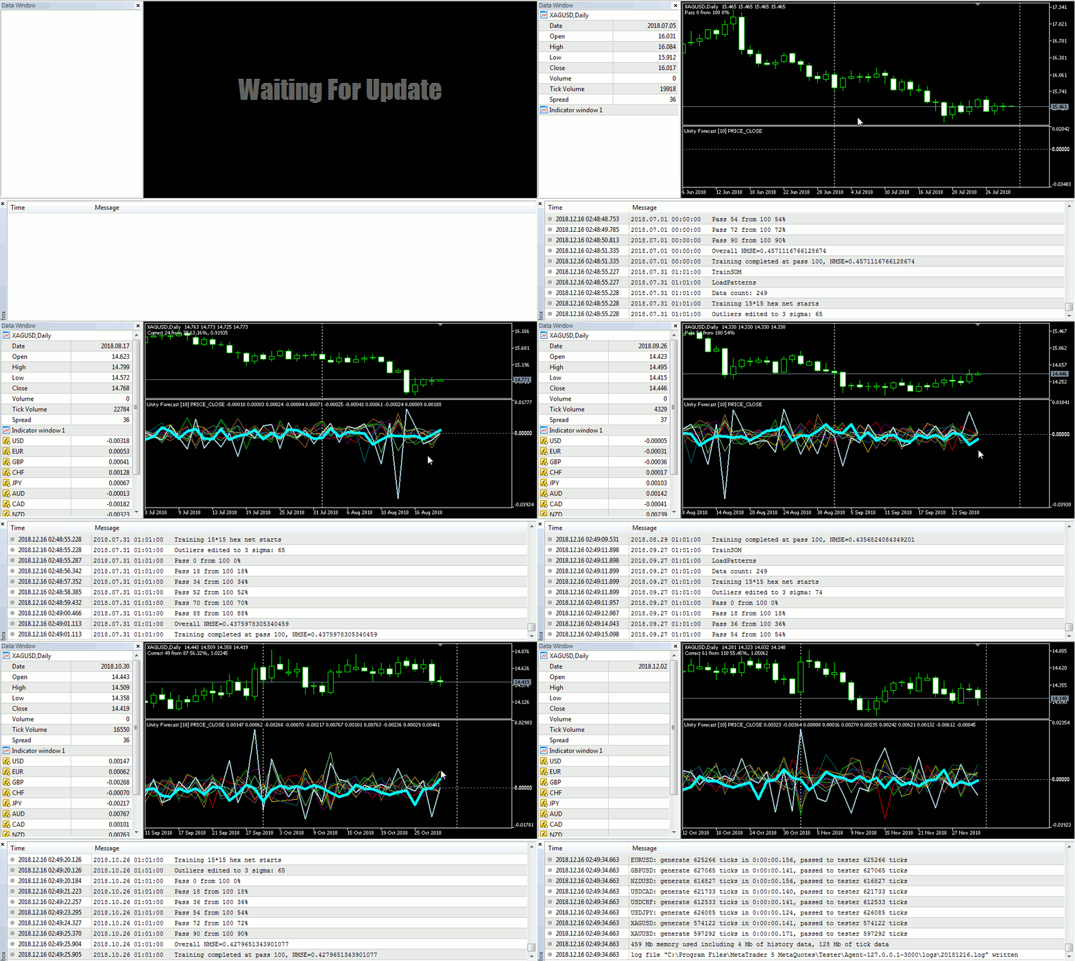
Unity-Forecast: Forecasting the movements of silver on the Forex and gold cluster in MetaTrader 5 Tester

At times, the accuracy reaches 60 %. We can conclude that, basically, the method works, if even it requires fundamentally selecting the forecasting object, preparing inputs, and long-time, meticulously configuring.

Attention! Training a network in the 'on-the-go' manner blocks the indicator (as well as other indicators with the same symbol/timeframe), which is not recommended. In the reality, this code shall be executed in an EA. Here, it is placed in an indicator for illustrative purposes. To update the network in the indicator, you can use a helping EA generating maps by schedule, while this indicator will reload them by the name specified in NetFileName.

The following options can be considered to enhance the forecasting quality: Adding external factors, such as week day numbers to the inputs or implementing more sophisticated methods based on several Kohonen networks or on a Kohonen network together with the networks of other types.

Conclusion

This article deals with the practical use of Kohonen networks in solving some problems of a trader. Neural network-based technology is a powerful and flexible tool allowing you to involve various data processing methods. At the same time, they require carefully selecting input variables, history depths, and combinations of parameters, so their successful use is largely determined by the user's expertise and skills. The classes considered herein allow you to test Kohonen networks in practice, gain the necessary experience in using them, and adapt them to your own tasks.