Practical Use of Kohonen Neural Networks in Algorithmic Trading. Part I. Tools

The subject of Kohonen neural networks was approached to in some articles on the mql5.com website, such as Using Self-Organizing Feature Maps (Kohonen Maps) in MetaTrader 5 and Self-Organizing Feature Maps (Kohonen Maps) - Revisiting the Subject. They introduced readers to the general principles of building neural networks of this type and visually analyzing the economic numbers of markets using such maps.

However, in practical terms, using Kohonen networks just for algorithmic trading has been confined with only one approach, namely the same visual analysis of topology maps built for the EA optimization results. In this case, one's value judgment, or rather one's vision and ability to draw reasonable conclusions from a picture turns out to be, perhaps, the crucial factor, sidelining the network properties regarding representing data in terms of nuts-and-bolts matters.

In other words, the features of neural network algorithms were not used to the full, i.e., they were used without automatically extracting knowledge or supporting decision making with specific recommendations. In this paper, we consider the problem of defining the optimal sets of robots' parameters in a more formalized manner. Moreover, we are going to apply Kohonen network to forecasting economic ranges. However, before proceeding to these applied problems, we should revise the existing source codes, get something fixed, and make some improvements.

It is highly recommended to read the above articles first, if you are not familiar with the terms such as 'network', 'layer', 'neuron' ('node'), 'link', 'weight', 'learning rate', 'learning range', and other notions related to Kohonen networks. Then we will have to saturate ourselves in this matter, so re-teaching the basic notions would lengthen this publication significantly.

Correcting the Errors

We are going to invoke classes CSOM and CSOMNode published in the former of the above articles, with an eye to the additions to the latter one. The key code fragments in them are practically identical and inherit the same problems.

First of all, it should be noted that, for some reason, neurons in the above classes are indexed, i.e. identified and defined with constructor parameters, by pixel coordinates. This is not very logical and complicates calculations and debugging at some points. Particularly under this approach, presentation settings affect calculations. Just imagine: There are two completely similar networks with the lattices sized identically, and they are learning using the same data set and having the same settings and random data generator initialization. However, the results obtained are different, just because the images of one network are larger than those of the another one. This is a mistake.

We will go to indexing neurons by numbers: Each neuron will have in array m_node (class CSOM) coordinates x and y corresponding with the column and row numbers, respectively, in the output layer of Kohonen network. Each neuron will be initialized using the CSOMNode::InitNode(x, y) method instead of the CSOMNode::InitNode(x1, y1, x2, y2) method. When we go to visualizing, the neuron coordinates will remain unchanged on changing the map size in pixels.

In inherited source codes, no input data normalization is used. However, it is very important in case where different components (features) of input vectors have different ranges of values. And this is the case in the EAs' optimization results and in pooling the data of different indicators. As to the optimization results, we can see there that the values having the total profits of dozens of thousands rub shoulders with small values, such as the fractions of Sharp ratio or the one-digit values of the restitution factor.

You should not teach a Kohonen network using such different-scale data, since the network would practically consider the larger components only and ignore the smaller ones. You can see this in the image below obtained using the program that we are going to consider in a step-wise manner within this article and attach hereto in the end. The program allows generating random input vectors, in which three components are defined within the ranges of [0, 1000], [0, 1], and [-1, +1], respectively. A special input, UseNormalization, allows enabling/disabling normalization.

Let us have a look at the final structure of the Kohonen network in three planes relevant to three dimensions of the vectors. First, the network learning result without normalization.

Kohonen network learning result without normalizing the inputs

Now, the same with normalization.

Kohonen network learning result with normalizing the inputs

The degree of the neuron weight adaptation is proportional to color gradient. Obviously, in no-normalization conditions, the network has learned the topological partitioning (classifying) in the first plane only, while the second and the third components are filled with minor noise. That is, the analytic capabilities of the network have been realized as little as to their one third. With normalization enabled, the spatial arrangement is visible in all the three planes.

Many ways of normalizing are known, but the most popular one is, perhaps, subtracting the mean value of the entire selection from each component, followed by dividing it by the standard deviation, i.e., sigma or root mean square. This sets the mean value of the transformed data to zero, and the standard deviation to unity.

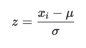 (1)

This technique is used in the updated class of CSOM, in method Normalize. It is clear that you should first calculate the mean values and sigmas for each component of the input data set, which is done in method InitNormalization (see below).

Canonical formulas for calculating the mean values and standard deviation mean using a two-run algorithm: The mean value should be found first, and then it is used in calculating the sigma.

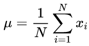                             (2)

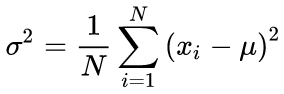     (3)

In our source code, we use a one-run algorithm based on the formula below:

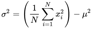 (4)

Obviously, normalization at the entry requires an opposite operation — denormalization — at the exit, that is, at transforming the output values of the network to the range of real values. this is done by method CSOM::Denormalize.

Since the normalized values fall symmetrically in the neighborhood of zero, we are going to change the initialization principle of neuron weights before starting to teach the network — instead of range [0, 1], it is range [-1, +1] now (see method CSOMNode::InitNode). This will enhance the efficiency of network learning.

Another aspect to be corrected is counting the learning iterations. In source classes, iteration shall be understood to mean specifying each individual input vector for the network. Therefore, the number of iterations should be corrected based on and in accordance with the size of the teaching selection. Recall that the Kohonen network learning and information fusion principle assumes that each sample is specified for the network quite a number of times. For example, if there are 100 entries in the selection, then the number of iterations equaling to 10000 will have to be specified 100 times each, in average. However, if the selection makes 1000 entries, then the number of iterations must become 100000. A more convenient and conventional method is defining the number of so-called 'learning epoch', i.e., cycles within each of which all samples are fed to the network input randomly. this number will be set in parameter EpochNumber. Due to introducing it, the learning duration is parametrically detached from the size of the data set.

This is even more important, since the total input set can be divided into 2 components: The selection that teaches and the so-called validating selection. The latter one is used to track the network learning quality. The matter is that adapting the network to the inputs during teaching it has a "flip side": The network starts adapting to the characteristics of specific samples and, doing so, loses its ability to generalize and work adequately on unknown data (other than that used for teaching). After all, the idea of learning, as a rule, consists in the ability of the characteristics detected using the network to be applied in future.

In the program under consideration, input parameter ValidationSetPercent is responsible for enabling the validation. By default, it is equal to 0, and all data is used for learning. If we specify, say, 10 there, then only 90 % of the samples are used for learning, while for the remaining 10 % the Normalized Mean Squared Error is calculated on each iteration (epoch), and learning process stops at the moment where the error starts growing.

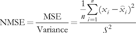 (5)

Normalization consists in dividing the mean squared error by the dispersion of data itself, which results in that the index is always below 1. When considering each vector separately, this mean squared error is, in fact, a quantization error, since it is based on the difference between its components and the weights of the relevant neural synapses, giving the best approximation of this vector among all neurons. We should recall that this winning neuron is called BMU (best matching unit) or BMN (best matching node) in Kohonen networks — in class CSOM, the GetBestMatchingNode method and similar techniques are responsible for searching it.

With validation enabled, the number of iterations will exceed that specified in parameter EpochNumber. Due to the special features of the Kohonen network architecture, validation can only be performed after the network has passed the self-organizing phase on EpochNumber epochs. On completion of that phase, the learning rate and scope reduce so significantly that the fine tuning of weights starts and then the convergence phase begins. It is here where the "early stop" of learning is applied using the validation set.

Whether to use validation or not, depends on the specificity of the problem. Besides, the validation set can be used to match the network size. For the purpose of this article, we are not going to get into this matter. We are just using the well-known empiric rule relating the network size to the number of teaching data:

N ~ 5 * sqrt(M)          (6)

where N is the number of neurons within the network, and M is the number of input vectors. For a Kohonen network with the square output layer, we get the size:

S = sqrt(5 * sqrt(M))  (7)

where S is the number of neurons vertically and horizontally. We will introduce this value into parameters CellsX and CellsY.

The last issue to be corrected in the original source codes is related to processing the hexagonal grid. Kohonen maps are known to be built using the rectangular or hexagonal placement of cells (neurons), and both modes are initially realized in source codes. However, the hexagonal grid is just displayed as hexagonal cells, but is calculated completely as the rectangular one. To get to the root of the error here, let us consider the following illustration.

Geometry of the neuron neighborhood in a rectangular and a hexagonal grid

The logic surrounding of a random neuron is shown here (with the coordinates of 3;3, in this case) for the grids of both geometries. Surrounding radius is 1. In the square grid, the neuron has 4 direct neighbors, while it has 6 ones in the hexagonal grid. Realization of the tessellation appearance is achieved by shifting every alternate string of cells by a half-cell aside. However, this does not change their internal coordinates, and, in terms of algorithm, the neuron surrounding in the hexagonal grid appears as before — it is marked in pink.

Apparently, this is wrong and should be corrected by including neurons highlighted in yellow.

Formally, the algorithm calculates the surrounding both using the adjacent neighbors and as convex decreasing radial function depending on the distance between the coordinates of cells. In other words, neighborhood is not a binary property of a neuron (either a neighbor or not), but a continuous quantity calculated by Gaussian formula:

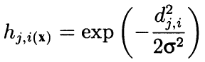 (8)

Here, dji is the distance between neurons j and i (continuous numbering is meant, not coordinates x and y); and sigma is the efficient width of the neighborhood or the learning radius that reduces gradually during learning. At the beginning of learning, the neighborhood covers with a symmetric "bell" a much larger space than the immediately adjacent neurons.

Since this formula depends on distances, it also misrepresents the neighborhood, is the coordinates have not been corrected properly. Therefore, the following source code strings from method CSOM::Train:

      for(int i = 0; i < total_nodes; i++)
      {
         double DistToNodeSqr = (m_som_nodes[winningnode].X() - m_som_nodes[i].X()) * (m_som_nodes[winningnode].X() - m_som_nodes[i].X())
                              + (m_som_nodes[winningnode].Y() - m_som_nodes[i].Y()) * (m_som_nodes[winningnode].Y() - m_som_nodes[i].Y());

have been complemented:

      bool odd = ((winningnode % m_ycells) % 2) == 1;
      for(int i = 0; i < total_nodes; i++)
      {
        bool odd_i = ((i % m_ycells) % 2) == 1;
        double shiftx = 0;

        if(m_hexCells && odd != odd_i)
        {
          if(odd && !odd_i)
          {
            shiftx = +0.5;
          }
          else // vice versa (!odd && odd_i)
          {
            shiftx = -0.5;
          }
        }
        double DistToNodeSqr = (m_node[winningnode].GetX() - (m_node[i].GetX() + shiftx)) * (m_node[winningnode].GetX() - (m_node[i].GetX() + shiftx))
                             + (m_node[winningnode].GetY() - m_node[i].GetY()) * (m_node[winningnode].GetY() - m_node[i].GetY());

The direction of correction 'shiftx' depends on the ratio of the properties of being even or odd of the rows where there are two neurons, between which the distance is calculated. If the neurons are in equally leveled rows, then there is no correction. If the winning neuron is in an odd row, then the even rows appear as shifted by a half-cell to the right from it, therefore, shiftx is equal to +0.5. If the winning neuron is in an even row, then the odd rows appear as shifted by a half-cell to the left of it, therefore, shiftx is equal to -0.5.

Now, it is especially important to pay attention to the following original strings:

        if(DistToNodeSqr < WS)
        {
          double influence = MathExp(-DistToNodeSqr / (2 * WS));
          m_node[i].AdjustWeights(data, learning_rate, influence);
        }

In fact, this conditional operator ensures some acceleration in calculations due to neglecting the neurons beyond the neighborhood of one sigma. However, in terms of learning quality, Gaussian formula is ideal, and such an intervention is unreasonable. If the too far neurons should be neglected, then for three sigmas, not just one. It is even more critical, after we have corrected the calculations of hexagonal grid, since the distance between the adjacent neurons located in neighboring rows is equal to sqrt(1*1 + 0.5*0.5) = 1.118, that is, above 1. In the source codes attached, this conditional operator is commented. If you really need to accelerate your calculations, use option:

        if(DistToNodeSqr < 9 * WS)

Attention! Due to the above nuance in the difference of distances between neighboring neurons depending on their row (single-row ones have a distance of 1, while those having adjacent rows have that of 1.118), the current realization is still non-ideal and suggests further correcting to achieve complete anisotropy.

Visualization

Notwithstanding that Kohonen networks are primarily associated with a visible graphic map, their topology and learning algorithms can perfectly work without any user interface. Particularly, the problems of forecasting or compacting the information doe not require any necessary visual analysis, and the classification of images can deliver a result as a number, i. e., the number of a class or of a probability of an event. Therefore, the functionality of Kohonen networks was divided between two classes. In class CSOM, only calculations, data loading and storing, and networks loading and storing have remained. In addition thereto, the derived class of CSOMDisplay was created, where all graphics had been placed. In my opinion, this is a simpler and more logical hierarchy than that proposed in article 2. In future, we are going to use CSOMDisplay for solving the problem of choosing the optimal EA parameters, while CSOM will be used for forecasting.

It should be noted that the grid type feature, i. e., whether it is rectangular or hexagonal, belongs to the basic class, since it affects the calculations of distances. Along with the number of nodes in vertical and horizontal directions, as well as with the dimensions of the data input space, the grid type is a part of architecture and should be saved in the file. When downloading the network from file, all those parameters are read from there, not from the program settings. Other settings that only affect the visual representation, such as map sizes in pixels, displaying the cell boundaries, or showing the captions, are not saved in the network file and can be changed repeatedly and randomly for the network once taught.

It should be noted that none of the updated classes do not represent a graphical user interface with controls — all the settings are specified via the inputs of MQL programs. At the same time, class CSOMDisplay still realizes some useful features.

Recall that, in the preceding samples of how to work with Kohonen networks, there was input named MaxPictures. It persists in the new realization. It is passed as maxpict to method CSOMDisplay::Init and sets the number of the network maps (planes) displayed within one row in the chart. Operating this parameter together with the unified image sizes in ImageW and ImageH, we can find an option where all maps fit in the screen. However, when there are many maps, such as where you have to analyze many settings of an EA, their sizes require significant reduction, which is inconvenient. In such cases, you can activate a new mode using MaxPictures, setting the parameter to 0.

In this mode, map images are generated on the chart not as objects OBJ_BITMAP_LABEL aligned with pixel coordinates, but as objects OBJ_BITMAP aligned with the time scale. Sizes of such maps can be increased up to the full height of the chart, and you can scroll them using a common horizontal scrolling bar by dragging them with your mouse or wheel, or using your keyboard. Number of maps is not limited to the screen size anymore. However, you should make sure that the number of bars is sufficient.

Increasing map sizes allows us to study them in more details, especially that class CSOMDisplay optionally displays various information inside the cells, such as the synapse weight values of the relevant plane, number of hits of teaching set vectors, the mean value and the dispersion of the relevant feature values of all vectors that have hit the cell. This information is not displayed by default, but it is always available in pop-up tips that appear if you hold the mouse cursor over one cell or another. The name of the current plane and the neuron coordinates are also shown in the pop-up tips.

Moreover, a double-click on any neuron will highlight that neuron in the inverted color in the current map and in all other maps simultaneously. This allows us to visually compare the neuron activities by all features simultaneously.

And, finally, it should be noted that the entire graphics have been moved to standard class CCanvas. This releases the code from external dependencies, but it has also a side effect: Y coordinates are now counted in a top-down manner, not bottom-up as it was previously. This results in displaying the map legends with the component names and the ranges of their values above the maps, not below them. However, this change does not seem to be critical.

Improvements

Before we can approach to applied problems, it is required to make some improvements of neural network classes. In addition to standard maps representing the synapse weights in the 2D spaces of specific features, we will prepare the calculations and displays of some service maps that are a de facto standard for Kohonen networks. Looking ahead, we will say that we will need many of them at the stage of applied experiments.

Let us define the indexes of additional dimensions, there will be 5 of them in total.

#define EXTRA_DIMENSIONS 5
#define DIM_HITCOUNT (m_dimension + 0)
#define DIM_UMATRIX  (m_dimension + 1)
#define DIM_NODEMSE  (m_dimension + 2) // quantization errors per node: average variance (square of standard deviation)
#define DIM_CLUSTERS (m_dimension + 3)
#define DIM_OUTPUT   (m_dimension + 4)

U-Matrix

First of all, we are going to calculate U-matrix, a unified matrix of distances, to evaluate the topology generated in the process of learning within the network. For each neuron in the network, this matrix contains the average distance between this neuron and its immediate neighbors. Since Kohonen network displays a multidimensional space of features into the two-dimensional space of the map. Folds occur in this two-dimensional space. In other words, despite the Kohonen network's property of keeping the arrangement inherent to the initial space, it is equally unachievable across the entire 2D space, and the geographical proximity of neurons becomes illusory. It is exactly U-matrix that is used to detect such areas. In it, the areas where there is a large difference between neuron weights and the weights of its neighbors appear as "peaks", while the areas where neurons are very similar look as "lowlands."

To calculate the distance between the neuron and the feature vector, there is method CSOMNode::CalculateDistance. We will create for it a counterpart method that will take the pointer to another neuron instead of the vector (array 'double').

double CSOMNode::CalculateDistance(const CSOMNode *other) const
{
  double vector[];
  other.GetCodeVector(vector);
  return CalculateDistance(vector);
}

Here, method GetCodeVector gets the array of the weights of another neuron and sends it immediately to calculating the distance in a common manner.

To get the unified neuron distance, it is necessary to calculate the distances to all its neighboring neurons and average them. Since the traversal of the neighboring neurons is a common task for several operations with the network grid, we will create a base class for traversal and then implement individual algorithms in its descendants, including summing up the distances.

#define NBH_SQUARE_SIZE    4
#define NBH_HEXAGONAL_SIZE 6

template<typename T>
class Neighbourhood
{
  protected:
    int neighbours[];
    int nbhsize;
    bool hex;
    int m_ycells;

  public:
    Neighbourhood(const bool _hex, const int ysize)
    {
      hex = _hex;
      m_ycells = ysize;

      if(hex)
      {
        nbhsize = NBH_HEXAGONAL_SIZE;
        ArrayResize(neighbours, NBH_HEXAGONAL_SIZE);
        neighbours[0] = -1; // up (visually)
        neighbours[1] = +1; // down (visually)
        neighbours[2] = -m_ycells; // left
        neighbours[3] = +m_ycells; // right
        /* template, applied dynamically in the loop below
        // odd row
        neighbours[4] = -m_ycells - 1; // left-up
        neighbours[5] = -m_ycells + 1; // left-down
        // even row
        neighbours[4] = +m_ycells - 1; // right-up
        neighbours[5] = +m_ycells + 1; // right-down
        */
      }
      else
      {
        nbhsize = NBH_SQUARE_SIZE;
        ArrayResize(neighbours, NBH_SQUARE_SIZE);
        neighbours[0] = -1; // up (visually)
        neighbours[1] = +1; // down (visually)
        neighbours[2] = -m_ycells; // left
        neighbours[3] = +m_ycells; // right
      }
    
    }
    ~Neighbourhood()
    {
      ArrayResize(neighbours, 0);
    }

    T loop(const int ind, const CSOMNode &p_node[])
    {
      int nodes = ArraySize(p_node);
      int j = ind % m_ycells;
      
      if(hex)
      {
        int oddy = ((j % 2) == 1) ? -1 : +1;
        neighbours[4] = oddy * m_ycells - 1;
        neighbours[5] = oddy * m_ycells + 1;
      }
      
      reset();

      for(int k = 0; k < nbhsize; k++)
      {
        if(ind + neighbours[k] >= 0 && ind + neighbours[k] < nodes)
        {
          // skip wrapping edges
          if(j == 0) // upper row
          {
            if(k == 0 || k == 4) continue;
          }
          else if(j == m_ycells - 1) // bottom row
          {
            if(k == 1 || k == 5) continue;
          }
          
          iterate(p_node[ind], p_node[ind + neighbours[k]]);
        }
      }
      
      return getResult();
    }
    
    virtual void reset() = 0;
    virtual void iterate(const CSOMNode &node1, const CSOMNode &node2) = 0;
    virtual T getResult() const = 0;
};

Depending on the type of grid passed to the constructor, the number of neighbors, nbhsize, is taken as equal to 4 and 6. Increments of the numbers of neighboring neurons, as related to the current neuron, are stored by array 'neighbours'. For example, in a square grid, the upper neighbor is obtained by deducting a unity from and the lower neighbor by adding a unity to the neuron number. Left and right neighbors have numbers differing by the grid column height, so this value is passed to the constructor as ysize.

The actual traversal of neighbors is performed by method 'loop'. Class Neighbourhood does not include any array of neurons, so it is passed as a parameter to method 'loop'.

This method in the loop goes across array 'neighbours' and additionally checks that the number of the neighbor does not go beyond the grid, considering the increment. For all valid numbers, abstract method 'iterate' is called where the links to the current neuron and to one of the surrounding neurons are passed.

Abstract method 'reset' is called before the loop, and abstract method getResult is called after the loop. A set of three abstract methods allows preparing and performing in the descendant classes the enumerating of neighbors and generating the result. The 'loop' method construction concept corresponds with the known OOP designing pattern — Template Method. Here, we should distinguish the 'template' term in the own name of the pattern from the language pattern of templates, which is also used in class Neighbourhood, since it is a template one, i. e., it is parametrized by a certain variable type T. Particularly, the 'loop' method itself and method getResult return the value of the T type.

Based on class Neighbourhood, we will write a class to calculate the U-matrix.

class UMatrixNeighbourhood: public Neighbourhood<double>
{
  private:
    int n;
    double d;
    
  public:
    UMatrixNeighbourhood(const bool _hex, const int ysize): Neighbourhood(_hex, ysize)
    {
    }
    
    virtual void reset() override
    {
      n = 0;
      d = 0.0;
    }
    
    virtual void iterate(const CSOMNode &node1, const CSOMNode &node2) override
    {
      d += node1.CalculateDistance(&node2);
      n++;
    }
    
    virtual double getResult() const override
    {
      return d / n;
    }
};

Working type is double. Through he basic class, the calculations of the distance are quite transparent.

We are going to calculate the distances for the entire map in method CSOM::CalculateDistances.

void CSOM::CalculateDistances()
{
  UMatrixNeighbourhood umnh(m_hexCells, m_ycells);
  
  for(int i = 0; i < m_xcells * m_ycells; i++)
  {
    double d = umnh.loop(i, m_node);
    
    if(d > m_max[DIM_UMATRIX])
    {
      m_max[DIM_UMATRIX] = d;
    }
    
    m_node[i].SetDistance(d);
  }
}

The value of the unified distance is saved in the object of the neuron. Later, when displaying all the planes, we will be able to define the distance values in a standard manner using a color palette, having included into calculations an additional dimension, DIM_UMATRIX. To scale the palette correctly, we save in this method the highest value of the distance within the relevant element of array m_max (all the realization principles remain unchanged from the previous realizations).

Number of hits and quantization error

The next additional dimension will collect statistics of the number of learning vectors hits in specific neurons. In other words, it is the density of populating the neurons with applied data. The higher it is in a specific neuron, the more statistically reasonable its weighting factors are. In the network, neurons having minor or even zero data coverage may occur. It there are many of them, it may speak for the issues in selecting the network size or for twisting the topology in the 2D projection of the multidimensional space. Hits of the samples into a certain neuron are calculated by the method of:

void CSOMNode::RegisterPatternHit(const double &vector[])
{
  m_hitCount++;
  double e = 0;
  for(int i = 0; i < m_dimension; i++) 
  {
    m_sum[i] += vector[i];
    m_sumP2[i] += vector[i] * vector[i];
    e += (m_weights[i] - vector[i]) * (m_weights[i] - vector[i]);
  }
  m_mse += e / m_dimension;
}

Counting itself is performed in the first string of m_hitCount++, where the internal counter is increased. The remaining code performs other useful work to be discussed below.

We will call method RegisterPatternHit upon completion of learning from class CSOM where we are going to create a special method of statistical processing each vector.

double CSOM::AddPatternStats(const double &data[])
{
  static double vector[];
  ArrayCopy(vector, data);
  
  int ind = GetBestMatchingIndex(vector);
  
  m_node[ind].RegisterPatternHit(vector);

  double code[];
  m_node[ind].GetCodeVector(code);
  Denormalize(code);
  
  double mse = 0;
  
  for(int i = 0; i < m_dimension; i++)
  {
    mse += (data[i] - code[i]) * (data[i] - code[i]);
  }
  
  mse /= m_dimension;
  
  return mse;
}

As a digression, it should be noted that method GetBestMatchingIndex used here, as well as some other ones from the group of methods GetBestMatchingXYZ, normalizes the incoming data inside itself, for which reason it is necessary to pass to it a copy of the vector. Otherwise, fuzzy modification of source data would be possible in a calling code.

Along with recoding the hit, this method also calculates the quantization error for the current neuron and for the vector passed. For this purpose, from the winning neuron the so-called code vector is called for, i. e., the array of synapse weights, and the sum of squares of the component-wise differences between the weights and the input vector is calculated.

As to AddPatternStatsm it is called immediately from another method, CSOM::CalculateStats, that just arranges the loop for all inputs.

double CSOM::CalculateStats(const bool complete = true)
{
  double data[];
  ArrayResize(data, m_dimension);
  double trainedMSE = 0.0;
  
  for(int i = complete ? 0 : m_validationOffset; i < m_nSet; i++)
  {
    ArrayCopy(data, m_set, 0, m_dimension * i, m_dimension);
    trainedMSE += AddPatternStats(data, complete);
  }
  
  double nmse = trainedMSE / m_dataMSE;
  if(complete) Print("Overall NMSE=", nmse);

  return nmse;
}

This method sums up all the quantization errors and compares them to the input data dispersion in m_dataMSE — this is exactly the NMSE calculations described above within the context of validation and learning stoppage. This method mentions variable m_validationOffset specified in creating object CSOM based on whether it uses dividing the input data set by the learning and validating sub-sets.

You guessed it, method CalculateStats is called at each epoch inside the method of Train (if the convergence phase has already started), and we can judge by the value returned whether the overall network error has started to increase, i. e., whether it is time to stop.

Dispersion of m_dataMSE is calculated beforehand, using the method of:

void CSOM::CalculateDataMSE()
{
  double data[];

  m_dataMSE = 0.0;
  
  for(int i = m_validationOffset; i < m_nSet; i++)
  {
    ArrayCopy(data, m_set, 0, m_dimension * i, m_dimension);

    double mse = 0;
    for(int k = 0; k < m_dimension; k++)
    {
      mse += (data[k] - m_mean[k]) * (data[k] - m_mean[k]);
    }
    
    mse /= m_dimension;
    m_dataMSE += mse;
  }
}

We obtain the value of the average, m_mean, for each component at the data normalization stage already.

void CSOM::InitNormalization(const bool normalization = true)
{
  ArrayResize(m_max, m_dimension + EXTRA_DIMENSIONS);
  ArrayResize(m_min, m_dimension + EXTRA_DIMENSIONS);
  ArrayInitialize(m_max, 0);
  ArrayInitialize(m_min, 0);
  ArrayResize(m_mean, m_dimension);
  ArrayResize(m_sigma, m_dimension);

  for(int j = 0; j < m_dimension; j++)
  {
    double maxv = -DBL_MAX;
    double minv = +DBL_MAX;
    
    if(normalization)
    {
      m_mean[j] = 0;
      m_sigma[j] = 0;
    }
    
    for(int i = 0; i < m_nSet; i++)
    {
      double v = m_set[m_dimension * i + j];
      if(v > maxv) maxv = v;
      if(v < minv) minv = v;
      if(normalization)
      {
        m_mean[j] += v;
        m_sigma[j] += v * v;
      }
    }
    
    m_max[j] = maxv;
    m_min[j] = minv;
    
    if(normalization && m_nSet > 0)
    {
      m_mean[j] /= m_nSet;
      m_sigma[j] = MathSqrt(m_sigma[j] / m_nSet - m_mean[j] * m_mean[j]);
    }
    else
    {
      m_mean[j] = 0;
      m_sigma[j] = 1;
    }
  }
}

Turning to additional planes, it should be noted that, upon having calculated in CSOMNode::RegisterPatternHit, each neuron is able to return the relevant statistics using the methods of:

int CSOMNode::GetHitsCount() const
{
  return m_hitCount;
}

double CSOMNode::GetHitsMean(const int plane) const
{
  if(m_hitCount == 0) return 0;
  return m_sum[plane] / m_hitCount;
}

double CSOMNode::GetHitsDeviation(const int plane) const
{
  if(m_hitCount == 0) return 0;
  double z = m_sumP2[plane] / m_hitCount - m_sum[plane] / m_hitCount * m_sum[plane] / m_hitCount;
  if(z < 0) return 0;
  return MathSqrt(z);
}

double CSOMNode::GetMSE() const
{
  if(m_hitCount == 0) return 0;
  return m_mse / m_hitCount;
}

Thus, we obtain the data to fill two planes — with the number of the displays of input vectors by neurons and with the quantization error.

Network response

The next additional plane will be the yield map and network response to a specific sample. It should be recalled that, upon feeding a signal to the network, along with the winning neuron, all other neurons are activated to a greater of lesser extent. the possibility to compare the active response excursion can help in defining the stability of the solution proposed by the network.

Network response calculations are maximally simple. In class CSOMNode, we will write the method of:

double CSOMNode::CalculateOutput(const double &vector[])
{
  m_output = CalculateDistance(vector);
  return m_output;
}

And we will call it for each neuron in the network class.

void CSOM::CalculateOutput(const double &vector[], const bool normalize = false)
{
  double temp[];
  ArrayCopy(temp, vector);
  if(normalize) Normalize(temp);
  m_min[DIM_OUTPUT] = DBL_MAX;
  m_max[DIM_OUTPUT] = -DBL_MAX;
  for(int i = 0; i < ArraySize(m_node); i++)
  {
    double x = m_node[i].CalculateOutput(temp);
    if(x < m_min[DIM_OUTPUT]) m_min[DIM_OUTPUT] = x;
    if(x > m_max[DIM_OUTPUT]) m_max[DIM_OUTPUT] = x;
  }
}

If the test vector is not provided to the program, the response is calculated by default, i.e., for the zero vector.

Clusterization

Finally, the last of the planes considered, but probably the most important one, will be cluster map. Arranging the input data on a two-dimensional map is just a half of the battle. the real purpose of the analysis is detecting the features and categorizing them into classes easy to understand in terms of application. Where the dimensions of the features space are relatively small, we can rather easily distinguish the areas having the required characteristics by colored spots on individual planes, those spots usually being isolated. However, with the expansion of the input data structure, the picture becomes more complicated, and, instead of cross-analyzing a dozen of maps with different indexes, it is much more convenient to have one map divided into areas that claim attention.

Clusterization will result in both marking the map by areas having similar characteristics and identifying the centers of clusters. Then we can consider them as the most representative, in terms of statistics, samples of relevant classes. Here, we are gradually approaching the task of selecting the optimal EA parameters. However, we should implement clusterization.

K-Means

There are very many clusterization methods. The simplest option for MQL5 is to use the version of ALGLIB, which is included into the standard library. It is sufficient to include a header file:

#include <Math/Alglib/dataanalysis.mqh>

and write a method like this:

void CSOM::Clusterize(const int clusterNumber)
{
  int count = m_xcells * m_ycells;
  CMatrixDouble xy(count, m_dimension);
  int info;
  CMatrixDouble clusters;
  int membership[];
  double weights[];
  
  for(int i = 0; i < count; i++)
  {
    m_node[i].GetCodeVector(weights);
    xy[i] = weights;
  }

  CKMeans::KMeansGenerate(xy, count, m_dimension, clusterNumber, KMEANS_RETRY_NUMBER, info, clusters, membership);
  Print("KMeans result: ", info);
  if(info == 1) // ok
  {
    for(int i = 0; i < m_xcells * m_ycells; i++)
    {
      m_node[i].SetCluster(membership[i]);
    }
    
    ArrayResize(m_clusters, clusterNumber * m_dimension);
    for(int j = 0; j < clusterNumber; j++)
    {
      for(int i = 0; i < m_dimension; i++)
      {
        m_clusters[j * m_dimension + i] = clusters[i][j];
      }
    }
  }
}

It performs clusterization using algorithm K-Means. Unfortunately, as far as I know, it is the only clustering algorithm in the ALGLIB version in MQL5, although the latest version of the original library provides other ones, such as agglomerative hierarchic clustering.

"Unfortunately", because algorithm K-Means is the most "straight-line" one to some extent: Its essence reduces to searching for the centers of a given number of spheroids within the space of features, which cover the sampling points in the most efficient manner, i. e., the minimum of the sum of squares of the distances to the points from the cluster centers. the matter is that, due to their fixed forms, spheroids have some specific limitations regarding the separability of non-linear clusters. In principle, K-Means is a special case of algorithm Expectation Maximization that operates ellipsoids of different orientations and forms and, therefore, would be more preferable. However, even when using it, there is a probability of sticking in the local minimum, since both algorithms use convex forms and a random arrangement of the cluster centers only. Disadvantages can also include the fact that the number of clusters has to be specified beforehand.

However, let us consider how the clusterization is arranged using K-Means in ALGLIB. The main operation is performed by method CKMeans::KMeansGenerate. We pass to it an array with source data in a special object-based format (CMatrixDouble xy), number of vectors (count), dimensions of the feature space (m_dimension), and the desired number of clusters (clusterNumber), the latter one to be specified in the parameters of the MQL program. The next input, KMEANS_RETRY_NUMBER, is the number of iterations to be made by the algorithm with different, randomly selected initial centers, trying to avoid the local solution. In our case, it is a macro that is equal to 10. As the result of the function operation, we will obtain the execution code named 'info' (different values suggest success or an error), the object-based array named CMatrixDouble clusters with clusters coordinates, and the array of the inputs being the members of the clusters (membership).

We save the cluster centers in array m_clusters to mark them on the map, and we also color each neuron with a color relevant to its membership in the cluster:

m_node[i].SetCluster(membership[i]);

When working with ALGLIB, please keep in mind that it uses its own random number generator that considers the internal status of the special static object. Therefore, even an obvious initialization of the standard generator through MathSrand does not reset its status. This is especially critical for EAs, since global objects are not re-generated in them when changing the settings. As a result, the reproducibility of calculation results may turn out to be difficult with ALGLIB, if CMath::m_state is not reset to zero in OnInit.

Considering the above disadvantages of K-Means, it is desirable to have an alternative clusterization method. One alternative solution is plain to see.

Alternative

Let us turn our attention to Kohonen maps, particularly the additional dimensions we have introduced. U-Matrix is of particular interest. This plane shows the areas of the closest neurons, i.e., they are close both in terms of 2D-map topology and in terms of feature space. As we can remember, similar neurons for a kind of "lowlands" in U-Matrix. They are great candidates to become clusters.

We can transform the map of unified distances into clusters, for example, in the following manner.

Copy the information on all neurons into an array and sort it ascending by the value of the U-distance (CSOMNode::GetDistance()).

For a given neuron, we will check in the loop by array, whether the neighboring neurons belong to a cluster.

• If not, we create a new cluster and assign the current neuron to it. Note that the clusters will be created, starting with the zero index, which corresponds with the most "important" cluster, since it matches the minimum U-distance, and then further in the order of descending importance. In terms of U-distances, each successive cluster will be less compact.
• If among neighboring neurons there are those marked with a cluster, we will select among them the highest one, i. e., the one having the lowest index, and assign the current neuron to that cluster.

It is simple. Should not the neurons populating density be also considered? After all, U-distance has been differently supported for neurons having different numbers of hits. In other words, if two neurons have the same U-distance, the one of them, to which more samples have been displayed, must have the advantage of the neuron having a lower number.

Then it is sufficient to change the initial array sorting in the described algorithm in the order of the values in formula CSOMNode::GetDistance() / sqrt(CSOMNode::GetHitsCount()). I added square root to smooth its affect in case of a large population, while the smaller population should be "punished" stricter.

However, if we are using two service planes, then might it be reasonable to analyze the third one, i. e., that with the quantization error? Indeed, the larger the quantization error is in a specific neuron, the less we should trust in the information on the small U-distance in it, and vice versa.

If we remember how the function with a quantization error appears:

double CSOMNode::GetMSE() const
{
  if(m_hitCount == 0) return 0;
  return m_mse / m_hitCount;
}

then we will easily note that the m_hitCount counter of hits is used in it (in the denominator only). Therefore, we can re-write the preceding formula for sorting the array of neurons as CSOMNode::GetDistance() * MathSqrt(CSOMNode::.GetMSE()) — and then all the three additional indexes will be considered in it, which we have added to our Kohonen network realization.

We are almost ready to present the alternative clusterization algorithm in its final form, but one minor thing has remained. Inside the loop by the neurons array, we should check the neighborhood of the current neuron for the presence of neighboring clusters. A bit earlier, we implemented the template class, Neighbourhood, for the local overlook. Now, we are going to create its descendant focusing on searching for clusters.

class ClusterNeighbourhood: public Neighbourhood<int>
{
  private:
    int cluster;

  public:
    ClusterNeighbourhood(const bool _hex, const int ysize): Neighbourhood(_hex, ysize)
    {
    }
    
    virtual void reset() override
    {
      cluster = -1;
    }
    
    virtual void iterate(const CSOMNode &node1, const CSOMNode &node2) override
    {
      int x = node2.GetCluster();
      if(x > -1)
      {
        if(cluster != -1) cluster = MathMin(cluster, x);
        else cluster = x;
      }
    }
    
    virtual int getResult() const override
    {
      return cluster;
    }
};

The class contains the number of potential cluster (the number is an integer, so we parametrize the template with the int type). Initially, this variable is initialized in -1 within the reset method, i. e., there is no cluster. Then, with the parent class calling from its loop method our new realization 'iterate', we obtain the cluster number of each neighboring neuron, compare it to cluster, and save the minimum value. The same, or -1, if no clusters have been found, is returned by the method of getResult.

As an improvement, we propose to track the "peak height" between neurons, i. e., the value of node1.CalculateDistance(&node2)), and to perform the cluster number "flowing" from one neuron to another one, only if the "height" is lower than it was before. the final realization version is presented in the source code.

Finally, we can implement the alternative clusterization.

void CSOM::Clusterize()
{
  double array[][2];
  int n = m_xcells * m_ycells;
  ArrayResize(array, n);
  for(int i = 0; i < n; i++)
  {
    if(m_node[i].GetHitsCount() > 0)
    {
      array[i][0] = m_node[i].GetDistance() * MathSqrt(m_node[i].GetMSE());
    }
    else
    {
      array[i][0] = DBL_MAX;
    }
    array[i][1] = i;
    m_node[i].SetCluster(-1);
  }
  ArraySort(array);
  
  ClusterNeighbourhood clnh(m_hexCells, m_ycells);

  int count = 0; // number of clusters
  ArrayResize(m_clusters, 0);
  
  for(int i = 0; i < n; i++)
  {
    // skip if already assigned
    if(m_node[(int)array[i][1]].GetCluster() > -1) continue;
    
    // check if current node is adjacent to any existing cluster
    int r = clnh.loop((int)array[i][1], m_node);
    if(r > -1) // a neighbour belongs to a cluster already
    {
      m_node[(int)array[i][1]].SetCluster(r);
    }
    else // we need new cluster
    {
      ArrayResize(m_clusters, (count + 1) * m_dimension);
      
      double vector[];
      m_node[(int)array[i][1]].GetCodeVector(vector);
      ArrayCopy(m_clusters, vector, count * m_dimension, 0, m_dimension);
      
      m_node[(int)array[i][1]].SetCluster(count++);
    }
  }
}

The algorithm follows practically fully the verbal pseudocode described above: We fill the two-dimensional array (the value from the formula in the first dimension, and the neuron index in the second one), sort, visit all the neurons in the loop, and analyze the neighborhood for each of them.

Quality of clusterization should, of course, be evaluated in practice, and I presuppose the presence of topological issues. However, considering that the most of the classical clusterization methods also have problems and are inferior in easiness to the proposed one, the new solution looks attractively.

Among the advantages of this realization, I would mention the fact that clusters are arranged by their importance (in the above-mentioned K-Means, clusters are equal), their form is random, and the number does not need to be pre-defined. It should be noted that the last one has a reverse side, i. e., the number of clusters can be rather large. Along that, the arrangement of clusters by the content similarity degree and minimum error allows practically considering only the first 5-10 clusters and leaving the other ones "behind the scenes."

Since I have not found any similar clusterization method in any open sources, I propose to name it Korotky clusterization, or longer but decent — short-path clusterization, based on U-Matrix and quantization error (QE).

Running ahead, I should say that, upon many tests, it was practically fortified that the cluster centers found by algorithm K-Means provided worse results than the alternative clusterization (at least in the problem of analyzing the optimization results). So, only that method of clusterization will be meant and applied hereinafter.

Testing

It's time to move from theory to practice and to test out how the network works. Let us create a simple, universal Expert Advisor with the options of demonstrating the basic functionality. We will name it SOM-Explorer.

Let us include header files with the above classes. Define the inputs.

Group — Network Structure and Data Settings

• DataFileName — the name of a text file with the data for teaching or testing; class CSOM supports format csv, but we will add reading set-files in the EA itself a bit later, since the analysis of optimizing settings of other EAs is "at stake"; where the file containing inputs is specified, its name is also used to save the network after having taught it, but with another extension (see below); you can indicate or not the csv extension; and the name may include a folder inside MQL5/Files;
  
  
• NetFileName — the name of a binary file of its own format with extension som; class CSOM is able to save and read the networks in/from such files; if somebody needs changing the structure of data to be stored, then change the version number in the signature that is written in the beginning of the file; if NetFileName is empty, the EA works in the learning mode, while if the network is specified, then in the testing mode, i. e., displaying the inputs into the ready network; you can indicate or not the som extension; and the name may include a folder inside MQL5/Files;
  
  
• if both DataFileName and NetFileName are empty, the EA will generate a demonstration set of random 3D-data and perform teaching on it;
  
  
• if the network name in NetFileName is correct, you can indicate in DataFileName the name of a non-existing file, such as just the '?' character, which leads to the EA generating a random sample of test data for the range of definitions that is saved in the network file (note that this information is necessary for the taught network to correctly normalize the unknown data in operating mode; feeding the network input with the values from another range of definitions will not, of course, lead to a fallout, but the results will be unreliable; for example, it is difficult to expect the network to work properly, if a negative value of drawdown or of the number of deals is provided to it.
  
  
• CellsX — horizontal size of the grid (number of neurons), 10 by default;
  
  
• CellsY — vertical size if the grid (number of neurons), 10 by default;
  
  
• HexagonalCell — the feature of using a hexagonal grid, it is 'true' by default; for a rectangular grid, switch to 'false';
  
  
• UseNormalization — enabling/disabling normalization for inputs; it is 'true' by default, and it is recommended not to disable it;
  
  
• EpochNumber — the number of learning epochs; 100 by default;
  
  
• ValidationSetPercent — the size of validation selection in percentage of the total number of inputs; it is 0 by default, i. e., validation is disabled; in case of using it, the recommended value is around 10;
  
  
• ClusterNumber — the number of clusters; it is 1 by default, which means our adaptive clusterization; the value of 0 disables clusterization; values above 0 launch clusterization using the K-Means method; clusterization is performed immediately after learning; and clusters are saved to the network file;

Group - Visualization

• ImageW — the horizontal size of each map (plane) in pixels, 500 by default;
  
  
• ImageH — the vertical size of each map (plane) in pixels, 500 by default;
  
  
• MaxPictures — the number of maps in a row; it is 0 by default, which means the mode of displaying the maps in a continuous row with the scrolling option (large images are allowed); if MaxPictures is above 0, then the entire set of planes is displayed in several rows, in each of which the MaxPictures of the maps is located (it is convenient in viewing all maps together in a small scale);
  
  
• ShowBorders — enabling/disabling drawing the borders between neurons; it is 'false' by default;
  
  
• ShowTitles — enabling/disabling displaying the texts with neuron characteristics, it is 'true' by default;
  
  
• ColorScheme — selecting one of 4 color schemes; it is Blue_Green_Red (the most colorful one) by default;
  
  
• ShowProgress — enabling/disabling dynamically updating the network images during learning; it is performed 1 time a second; it is 'true' by default;

Group - Options

• RandomSeed — an integer for initializing the random number generator; it is 0 by default;
• SaveImages — the option of saving the network images upon completion; it can also be used after learning and after the first launch; it is 'false' by default;

These are just basic settings. As we continue solving the problems, we will add some other specific parameters.

Note! The EA changes the settings of the current chart — open a new chart dedicated for working with this EA only.

CSOMDisplay class object will perform all the work in the EA.

CSOMDisplay KohonenMap;

During initialization, do not forget to enable mouse movement events processing — the class uses them to display pop-up tips and for scrolling.

void OnInit()
{
  ChartSetInteger(0, CHART_EVENT_MOUSE_MOVE, true);
  EventSetMillisecondTimer(1);
}

void OnChartEvent(const int id, const long &lparam, const double &dparam, const string &sparam)
{
  KohonenMap.OnChartEvent(id, lparam, dparam, sparam);
}

Neural-network algorithms (learning or testing) shall be launched in the EA only once — by timer, and then the timer is disabled.

void OnTimer()
{
  EventKillTimer();
  
  MathSrand(RandomSeed);
  
  bool hasOneTestPattern = false;
  
  if(NetFileName != "")
  {
    if(!KohonenMap.Load(NetFileName)) return;
    KohonenMap.DisplayInit(ImageW, ImageH, MaxPictures, ColorScheme, ShowBorders, ShowTitles);

    Comment("Map ", NetFileName, " is loaded; size: ", KohonenMap.GetWidth(), "*", KohonenMap.GetHeight(), "; features: ", KohonenMap.GetFeatureCount());

If a ready file with the network is specified, we load it and prepare the display in accordance with visual settings.

    if(DataFileName != "")
    {
      if(!KohonenMap.LoadPatterns(DataFileName))
      {
        Print("Data loading error, file: ", DataFileName);

        // generate a random test vector
        int n = KohonenMap.GetFeatureCount();
        double min, max;
        double v[];
        ArrayResize(v, n);
        for(int i = 0; i < n; i++)
        {
          KohonenMap.GetFeatureBounds(i, min, max);
          v[i] = (max - min) * rand() / 32767 + min;
        }
        KohonenMap.AddPattern(v, "RANDOM");
        Print("Random Input:");
        ArrayPrint(v);
        double y[];
        CSOMNode *node = KohonenMap.GetBestMatchingFeatures(v, y);
        Print("Matched Node Output (", node.GetX(), ",", node.GetY(), "); Hits:", node.GetHitsCount(), "; Error:", node.GetMSE(),"; Cluster N", node.GetCluster(), ":");
        ArrayPrint(y);
        KohonenMap.CalculateOutput(v, true);
        hasOneTestPattern = true;
      }
    }

If a file with test details is specified, we try to load it. If it does not work, display a message in the log and generate a random testing data sample, v. The number of features (dimensions of vectors) and their allowed ranges shall be defined using methods GetFeatureCount and GetFeatureBounds. Then, by calling AddPattern, the sample is added to the working data set under the name of RANDOM.

This method would be suitable for forming teaching selections from data sources having unsupported formats, such as databases, and for filling them directly from indicators. In principle, in this specific case, adding a sample to a working set is only necessary for subsequently visualizing them on the map (shown below), while only one call, GetBestMatchingFeatures, is sufficient for finding the most suitable neuron in the network. This method from among several available GetBestMatchingXYZ methods allows us to obtain the relevant values of the winning neuron's features in array y. Finally, using CalculateOutput, we display the network response to the test sample in an additional plane.

We continue following the EA code.

  }
  else // a net file is not provided, so training is assumed
  {
    if(DataFileName == "")
    {
      // generate 3-d demo vectors with unscaled values {[0,+1000], [0,+1], [-1,+1]}
      // feed them to the net to compare results with and without normalization
      // NB. titles should be valid filenames for BMP
      string titles[] = {"R1000", "R1", "R2"};
      KohonenMap.AssignFeatureTitles(titles);
      double x[3];
      for(int i = 0; i < 1000; i++)
      {
        x[0] = 1000.0 * rand() / 32767;
        x[1] = 1.0 * rand() / 32767;
        x[2] = -2.0 * rand() / 32767 + 1.0;
        KohonenMap.AddPattern(x, StringFormat("%f %f %f", x[0], x[1], x[2]));
      }
    }

If the taught network is not specified, we assume the learning mode. Check whether there are any inputs. If not, we generate a random set of three-dimensional vectors, in which the first component is within the range of [0,+1000], the second one is within [0,+1], and the third one is within [-1,+1]. The names of components are passed to the network using AssignFeatureTitles, and the data — using AddPattern already known.

    else // a data file is provided
    {
      if(!KohonenMap.LoadPatterns(DataFileName))
      {
        Print("Data loading error, file: ", DataFileName);
        return;
      }
    }

If inputs come from a file, load this file. In case of an error, finish the work, since there is no network or data.

Further, we perform teaching and clusterization.

    KohonenMap.Init(CellsX, CellsY, ImageW, ImageH, MaxPictures, ColorScheme, HexagonalCell, ShowBorders, ShowTitles);
    
    if(ValidationSetPercent > 0 && ValidationSetPercent < 50)
    {
      KohonenMap.SetValidationSection((int)(KohonenMap.GetDataCount() * (1.0 - ValidationSetPercent / 100.0)));
    }

    KohonenMap.Train(EpochNumber, UseNormalization, ShowProgress);

    if(ClusterNumber > 1)
    {
      KohonenMap.Clusterize(ClusterNumber);
    }
    else
    {
      KohonenMap.Clusterize();
    }
  }

If the analysis of an individual test sample has not been specified (particularly, immediately after learning), we form the network response to the vector with zeros by default.

  if(!hasOneTestPattern)
  {
    double vector[];
    ArrayResize(vector, KohonenMap.GetFeatureCount());
    ArrayInitialize(vector, 0);
    KohonenMap.CalculateOutput(vector);
  }

Then we draw all the maps in the internal buffers of graphical resources — the color behind first:

  KohonenMap.Render(); // draw maps into internal BMP buffers

and then, captions:

  if(hasOneTestPattern)
    KohonenMap.ShowAllPatterns();
  else
    KohonenMap.ShowAllNodes(); // draw labels in cells in BMP buffers

Marking the clusters:

  if(ClusterNumber != 0)
  {
    KohonenMap.ShowClusters(); // mark clusters
  }

Show the buffers on the chart and, optionally, save the images to files:

  KohonenMap.ShowBMP(SaveImages); // display files as bitmap images on chart, optionally save into files

The files are placed in a separate folder with the same name as that of the network file, if provided, or the file with data, if provided. If the data file has not been specified and the network has learned on randomly generated data, the name of the som-file and the folders containing the images are formed using the SOM prefix and the current date and time.

Finally, save the taught network to a file. If the network name has already been specified in NetFileName, it means that the EA has worked in the testing mode, so we needn't save the network again.

  if(NetFileName == "")
  {
    KohonenMap.Save(KohonenMap.GetID());
  }
}

We will try to start the EA with generating the test random data. With all the default settings, other than the image downscales used to ensure that all the planes get onto the screenshot, ImageW = 230, ImageH = 230, MaxPictures = 3, we obtain the following picture:

Sample Kohonen maps for random 3D vectors

Here, service data is displayed in each neuron (you can see the details by pointing the mouse cursor), and the clusters found are marked.

In that process, the following information (cluster information is limited by five; you can change it in the source code) is displayed in the log:

Pass 0 from 1000 0%
Pass 78 from 1000 7%
Pass 157 from 1000 15%
Pass 232 from 1000 23%
Pass 310 from 1000 31%
Pass 389 from 1000 38%
Pass 468 from 1000 46%
Pass 550 from 1000 55%
Pass 631 from 1000 63%
Pass 710 from 1000 71%
Pass 790 from 1000 79%
Pass 870 from 1000 87%
Pass 951 from 1000 95%
Overall NMSE=0.09420336270396877
Training completed at pass 1000, NMSE=0.09420336270396877
Clusters [14]:
"R1000" "R1"    "R2"   
N0
754.83131   0.36778   0.25369
N1
341.39665   0.41402  -0.26702
N2
360.72925   0.86826  -0.69173
N3
798.15569   0.17846  -0.37911
N4
470.30648   0.52326   0.06442
Map file SOM-20181205-134437.som saved

If now we specify the name of the created SOM-20181205-134437.som file with the network in parameter NetFileName and '?' in parameter DataFileName, we will obtain the result of a test run for a random sample not from the learning set. To see the maps better, let us make their sizes larger and set MaxPictures to 0. 

Kohonen maps for the first two components of random 3D-vectors

A Kohonen map for the third component of random 3D-vectors and counter of hits

U-Matrix and quantization errors

Clusters and Kohonen network response to the test sample

The sample is marked with RANDOM. Tips on neurons pop up when pointed by the mouse cursor. Something like the following is displayed in the log:

FileOpen error ?.csv : 5004
Data loading error, file: ?
Random Input:
457.17510   0.29727   0.57621
Matched Node Output (8,3); Hits:5; Error:0.05246704285146882; Cluster N0:
497.20453   0.28675   0.53213

So, the tools for working with Kohonen network are ready. We can go to applied problems. We are going to get to grips with that within our second article.

Conclusions

The open realizations of Kohonen neural networks have already been available to the MetaTrader users for some years. We have fixed some errors in them, complemented with useful tools, and tested their operation using a special demo EA. Source codes allow you applying the classes for your own tasks; we will consider the relevant examples further — to be continued.