Econometric approach to finding market patterns: Autocorrelation, Heat Maps and Scatter Plots
Maxim Dmitrievsky | 2 April, 2020
A brief review of the previous material and the prerequisites for creating a new model
In the first article, we introduced the concept of market memory, which is determined as a long-term dependence of price increments of some order. Further we considered the concept of "seasonal patterns" which exist in the markets. Until now, these two concepts existed separately. The purpose of the article is to show that "market memory" is of seasonal nature, which is expressed through maximized correlation of increments of arbitrary order for closely located time intervals and through minimized correlation for distant time intervals.
Let's put forward the following hypothesis:
Correlation of price increments depends on the presence of seasonal patterns, as well as on the clustering of nearby increments.
Let's try to confirm or refute it in a free intuitive and slightly mathematical style.
Classical econometric approach to identifying patterns in price increments is Autocorrelation
According to the classical approach, the absence of patterns in price increments is determined through the absence of serial correlation. If there is no autocorrelation, the series of increments is considered random, while further search for patterns is believed to be ineffective.
Let's see an example of visual analysis of EURUSD increments using autocorrelation function. All the examples will be performed using IPython.
def standard_autocorrelation(symbol, lag):
    rates = pd.DataFrame(MT5CopyRatesRange(symbol, MT5_TIMEFRAME_H1, datetime(2015, 1, 1), datetime(2020, 1, 1)),
                         columns=['time', 'open', 'low', 'high', 'close', 'tick_volume', 'spread', 'real_volume'])
    rates = rates.drop(['open', 'low', 'high', 'tick_volume', 'spread', 'real_volume'], axis=1).set_index('time')
    rates = rates.diff(lag).dropna()
    from pandas.plotting import autocorrelation_plot
    plt.figure(figsize=(10, 5))
    autocorrelation_plot(rates)

standard_autocorrelation('EURUSD', 50)
This function converts H1 close prices to relevant differences with the specified period (lag 50 is used) and displays the autocorrelation chart.
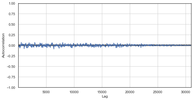
Fig. 1. Classical price increments correlogram
The autocorrelation chart does not reveal any patterns in price increments. Correlations between adjacent increments fluctuate around zero, which points to the randomness of the time series. We could end our econometric analysis right here, by concluding that the market is random. However, I suggest reviewing the autocorrelation function from a different angle: in the context of seasonal patterns.
I assumed that the correlation of price increments could be generated by the presence of seasonal patterns. Therefore, let us exclude from the example all hours except for a specific one. Thus, we will create a new time series, which will have its own specific properties. Build an autocorrelation function for this series:
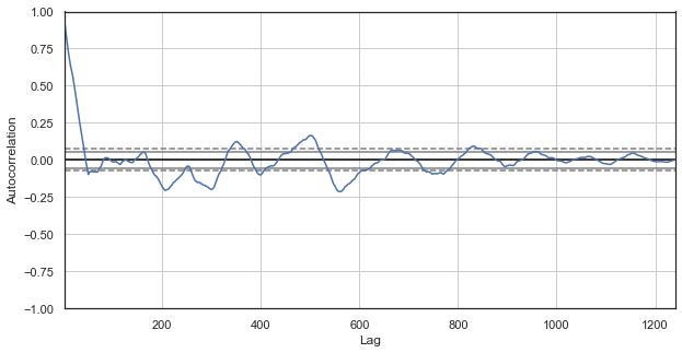
Fig. 2. A correlogram of price increments with excluded hours (with only the 1st hour for each day left)
The correlogram looks better for the new series. There is a strong dependence of current increments on previous ones. The dependence decreases when time delta between the increments increases. It means that current day 1st hour increment strongly correlates with the previous day's 1st hour increment, and so on. This very important information indicates the existence of seasonal patterns, i.e. increments have a memory.
Custom approach to identifying patterns in price increments is Seasonal Autocorrelation
We have found that there is a correlation between the current day's 1st hour increment and previous 1st hour increments, which however decreases, when the distance between the day increases. Now let's see if there is a correlation between the adjacent hours. For this purpose, let's modify the code:
def seasonal_autocorrelation(symbol, lag, hour1, hour2):
    rates = pd.DataFrame(MT5CopyRatesRange(symbol, MT5_TIMEFRAME_H1, datetime(2015, 1, 1), datetime(2020, 1, 1)),
                         columns=['time', 'open', 'low', 'high', 'close', 'tick_volume', 'spread', 'real_volume'])
    rates = rates.drop(['open', 'low', 'high', 'tick_volume', 'spread', 'real_volume'], axis=1).set_index('time')
    rates = rates.drop(rates.index[~rates.index.hour.isin([hour1, hour2])]).diff(lag).dropna()
    from pandas.plotting import autocorrelation_plot
    plt.figure(figsize=(10, 5))
    autocorrelation_plot(rates)

seasonal_autocorrelation('EURUSD', 50, 1, 2)
Here, delete all hours except the first and the second, then calculate the differences for the new series and build the autocorrelation function:
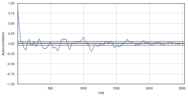
Fig. 3. A correlogram of price increments with excluded hours (with only the 1st and the 2nd hours for each day left)
Obviously, there is also a high correlation for the series of nearest hours, which indicates their correlation and mutual influence. Can we get a reliable relative score for all pairs of hours, not just for the selected ones? To do this, let's use the methods described below.
Heat map of seasonal correlations for all hours
Let's continue to explore the market and try to confirm the original hypothesis. Let's look at the big picture. The below function sequentially removes hours from the time series, leaving only one hour. It builds the price difference for this series and determines correlation with the series built for other hours:
#calculate correlation heatmap between all hours
def correlation_heatmap(symbol, lag, corrthresh):
    out = pd.DataFrame()
    rates = pd.DataFrame(MT5CopyRatesRange(symbol, MT5_TIMEFRAME_H1, datetime(2015, 1, 1), datetime(2020, 1, 1)),
                         columns=['time', 'open', 'low', 'high', 'close', 'tick_volume', 'spread', 'real_volume'])
    rates = rates.drop(['open', 'low', 'high', 'tick_volume', 'spread', 'real_volume'], axis=1).set_index('time')

    for i in range(24):
        ratesH = None
        ratesH = rates.drop(rates.index[~rates.index.hour.isin([i])]).diff(lag).dropna()
        out[str(i)] = ratesH['close'].reset_index(drop=True)
    plt.figure(figsize=(10, 10))
    corr = out.corr()
    # Generate a mask for the upper triangle
    mask = np.zeros_like(corr, dtype=np.bool)
    mask[np.triu_indices_from(mask)] = True
    sns.heatmap(corr[corr >= corrthresh], mask=mask)
    return out

out = correlation_heatmap(symbol='EURUSD', lag=25, corrthresh=0.9)
The function accepts the increment order (time lag), as well as the correlation threshold to drop off hours with low correlation. Here is the result:
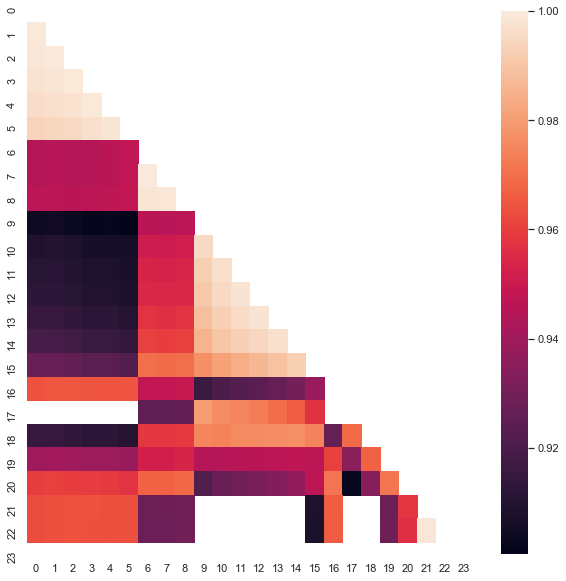
Fig. 4. Heat map of correlations between increments for different hours for the period 2015-2020.
It is clear that the following clusters have the maximum correlation: 0-5 and 10-14 hours. In the previous article we created a trading system based on the first cluster, which was discovered in a different way (using boxplot). Now the patterns are also visible on the heat map. Now let's view the second interesting cluster and analyze it. Here is the summary statistics for the cluster:
out[['10','11','12','13','14']].describe()
| 10 | 11 | 12 | 13 | ||
|---|---|---|---|---|---|
| count | 1265.000000 | 1265.000000 | 1265.000000 | 1265.000000 | 1265.000000 |
| mean | -0.001016 | -0.001015 | -0.001005 | -0.000992 | -0.000999 |
| std | 0.024613 | 0.024640 | 0.024578 | 0.024578 | 0.024511 |
| min | -0.082850 | -0.084550 | -0.086880 | -0.087510 | -0.087350 |
| 25% | -0.014970 | -0.015160 | -0.014660 | -0.014850 | -0.014820 |
| 50% | -0.000900 | -0.000860 | -0.001210 | -0.001350 | -0.001280 |
| 75% | 0.013460 | 0.013690 | 0.013760 | 0.014030 | 0.013690 |
| max | 0.082550 | 0.082920 | 0.085830 | 0.089030 | 0.086260 |
Parameters for all the cluster hours are quite close, however their average value for the analyzed sample is negative (about 100 five-digit points). A shift in average increments indicates that the market is more likely to decline during these hours than to grow. It is also worth noting that an increase in increments lag leads to a greater correlation between the hours due to the appearance of a trend component, while a decrease in the lag leads to lower values. However, the relative arrangement of clusters is almost unchanged.
For example, for a single lag, increments of hours 12, 13, and 14 still strongly correlate:
plt.figure(figsize=(10,5))
plt.plot(out[['12','13','14']])
plt.legend(out[['12','13','14']])
plt.show()
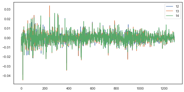
Fig. 5. Visual similarity between the series of increments with a single lag composed of different hours
Formula of regularity: simple but good
Remember the hypothesis:
Correlation of price increments depends on the presence of seasonal patterns, as well as on the clustering of nearby increments. f
We have seen in the autocorrelation diagram and on the heat map that there is a dependence of hourly increments both on past values and on nearby hour increments. The first phenomenon stems from the recurrence of events at certain hours of the day. The second one is connected with the clustering of volatility in certain time periods. Both of these phenomena should be considered separately and should be combined, if possible. In this article, we will perform an additional study of the dependence of particular hour increments (removing all other hours from the time series) on their previous values. The most interesting part of the research will be performed in the next article.
# calculate joinplot between real and predicted returns
def hourly_signals_statistics(symbol, lag,  hour, hour2, rfilter):
    rates = pd.DataFrame(MT5CopyRatesRange(symbol, MT5_TIMEFRAME_H1, datetime(2015, 1, 1), datetime(2020, 1, 1)),
                         columns=['time', 'open', 'low', 'high', 'close', 'tick_volume', 'spread', 'real_volume'])
    rates = rates.drop(['open', 'low', 'high', 'tick_volume', 'spread', 'real_volume'], axis=1).set_index('time')
# price differences for every hour series
    H = rates.drop(rates.index[~rates.index.hour.isin([hour])]).reset_index(drop=True).diff(lag).dropna()
    H2 = rates.drop(rates.index[~rates.index.hour.isin([hour2])]).reset_index(drop=True).diff(lag).dropna()
# current returns for both hours
    HF = H[1:].reset_index(drop=True); HL = H2[1:].reset_index(drop=True)
# previous returns for both hours
    HF2 = H[:-1].reset_index(drop=True); HL2 = H2[:-1].reset_index(drop=True)

# Basic equation:  ret[-1] = ret[0] - (ret[lag] - ret[lag-1])
# or Close[-1] = (Close[0]-Close[lag]) - ((Close[lag]-Close[lag*2]) - (Close[lag-1]-Close[lag*2-1]))

    predicted = HF-(HF2-HL2)
    real = HL
# correlation joinplot between two series
    outcorr = pd.DataFrame()
    outcorr['Hour ' + str(hour)] = H['close']
    outcorr['Hour ' + str(hour2)] = H2['close']
# real VS predicted prices
    out = pd.DataFrame()
    out['real'] = real['close']
    out['predicted'] = predicted['close']
    out = out.loc[((out['predicted'] >= rfilter) | (out['predicted'] <=- rfilter))]
# plptting results
    from scipy import stats
    sns.jointplot(x='Hour ' + str(hour), y='Hour ' + str(hour2), data=outcorr, kind="reg", height=7, ratio=6).annotate(stats.pearsonr)
    sns.jointplot(x='real', y='predicted', data=out, kind="reg", height=7, ratio=6).annotate(stats.pearsonr)

hourly_signals_statistics('EURUSD', lag=25, hour=13, hour2=14, rfilter=0.00)
Here is an explanation of what is done in the above listing. There are two series formed by removing unnecessary hours, based on which price increments (their difference) are calculated. Hours for the series are determined in the "hour" and "hour2" parameters. Then we obtain sequences with a lag of 1 for each hour, i.e. HF series is ahead of HL by one value — this allows calculating the actual increment and the predicted increment, as well as the difference between them. Firstly, let's construct a scatter plot for the 1st and 2nd hour increments:
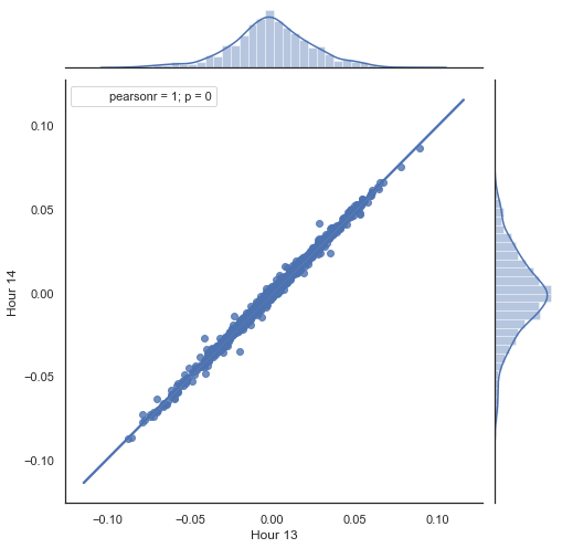
Figure 5. Scatter plot for increments of hour 13 and 14 for the period 2015-2020.
As expected, increments are highly correlated. Now let's try to predict the next increment based on the previous one. To do this, here is a simple formula, which can predict the next value:
Basic equation: ret[-1] = ret[0] - (ret[lag] - ret[lag-1])
or Close[-1] = (Close[0]-Close[lag]) - ((Close[lag]-Close[lag*2]) - (Close[lag-1]-Close[lag*2-1]))
Here is the explanation of the resulting formula. To predict the future increment, we are on the zero bar. Predict the value of the next increment ret[-1]. To do this, subtract the difference of the previous increment (with a 'lag') and the next one (lag-1) from the current increment. If the correlation of increments between two adjacent hours is strong, it can be expected that the predicted increment will be described by this equation. Below is an explanation of the equation for close prices. Thus, the future forecast is based on three increments. The second code part predicts future increments and compares them to actual ones. Here is a chart:
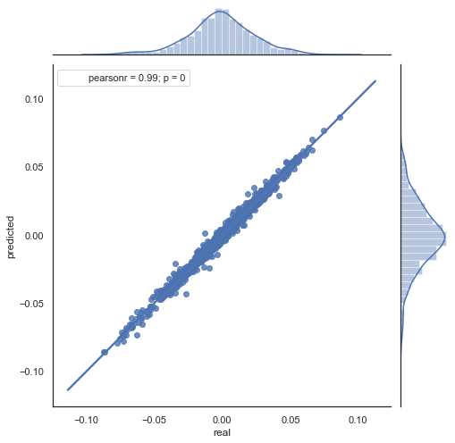
Figure 6. Scatter plot for actual and predicted increments for the period 2015-2020.
You can see that charts in figures 5 and 6 are similar. This means that the method for determining the patterns via correlation is adequate. At the same, values are scattered across the chart; they do not lie on the same line. These are forecast errors which negatively affect the prediction. They should be handled separately (which is beyond the scope of this article). Forecast around zero is not really interesting: if the forecast for the next price increment is equal to the current one, you cannot generate profit from it. Forecasts can be filtered using the rfilter parameter.
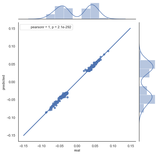
Figure 7. Scatter plot for actual and predicted increments with rfilter = 0.03 for the period 2015-2020.
Note that the heat map was created using data from 2015 to current date. Let us shift the starting day back to 2000:
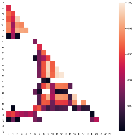
Fig. 8. Heat map of correlations between increments for different hours for the period from 2000 to 2020.
| 10 | 11 | 12 | 13 | ||
|---|---|---|---|---|---|
| count | 5151.000000 | 5151.000000 | 5151.000000 | 5151.000000 | 5151.000000 |
| mean | 0.000470 | 0.000470 | 0.000472 | 0.000472 | 0.000478 |
| std | 0.037784 | 0.037774 | 0.037732 | 0.037693 | 0.037699 |
| min | -0.221500 | -0.227600 | -0.222600 | -0.221100 | -0.216100 |
| 25% | -0.020500 | -0.020705 | -0.020800 | -0.020655 | -0.020600 |
| 50% | 0.000100 | 0.000100 | 0.000150 | 0.000100 | 0.000250 |
| 75% | 0.023500 | 0.023215 | 0.023500 | 0.023570 | 0.023420 |
| max | 0.213700 | 0.212200 | 0.210700 | 0.212600 | 0.208800 |
As you can see, the heat map is somewhat thinner, while the dependence between hours 13 and 14 has decreased. At the same time, the average value of increments is positive, which sets a higher priority to buying. A shift in the average value will not allow effectively trading in both time intervals, so you have to choose.
Let's look at the resulting scatter plot for this period (here I only provide the actual\forecast chart):
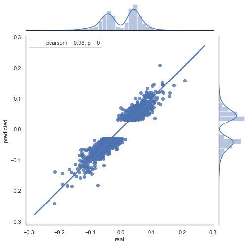
Fig. 9. Scatter plot for actual and forecast increments with rfilter = 0.03, for the period 2000 - 2020.
The spread of values has increased, which is a negative factor for such a long period.
Thus, we have obtained a formula and an approximate idea of the distribution of actual and predicted increments for certain hours. For greater clarity, the dependencies can be visualized in 3D.
# calculate joinplot between real an predicted returns
def hourly_signals_statistics3D(symbol, lag,  hour, hour2, rfilter):
    rates = pd.DataFrame(MT5CopyRatesRange(symbol, MT5_TIMEFRAME_H1, datetime(2015, 1, 1), datetime(2020, 1, 1)),
                         columns=['time', 'open', 'low', 'high', 'close', 'tick_volume', 'spread', 'real_volume'])
    rates = rates.drop(['open', 'low', 'high', 'tick_volume', 'spread', 'real_volume'], axis=1).set_index('time')
    rates = pd.DataFrame(rates['close'].diff(lag)).dropna()

    out = pd.DataFrame();
    for i in range(hour, hour2):
        H = None; H2 = None; HF = None; HL = None; HF2 = None; HL2 = None; predicted = None; real = None;
        H = rates.drop(rates.index[~rates.index.hour.isin([hour])]).reset_index(drop=True)
        H2 = rates.drop(rates.index[~rates.index.hour.isin([i+1])]).reset_index(drop=True)
        HF = H[1:].reset_index(drop=True); HL = H2[1:].reset_index(drop=True);     # current hours
        HF2 = H[:-1].reset_index(drop=True); HL2 = H2[:-1].reset_index(drop=True)  # last day hours

        predicted = HF-(HF2-HL2)
        real = HL

        out3D = pd.DataFrame()
        out3D['real'] = real['close']
        out3D['predicted'] = predicted['close']
        out3D['predictedABS'] = predicted['close'].abs()
        out3D['hour'] = i
        out3D = out3D.loc[((out3D['predicted'] >= rfilter) | (out3D['predicted'] <=- rfilter))]

        out = out.append(out3D)

    import plotly.express as px
    fig = px.scatter_3d(out, x='hour', y='predicted', z='real', size='predictedABS', color='hour', height=1000, width=1000)
    fig.show()

hourly_signals_statistics3D('EURUSD', lag=24, hour=10, hour2=23, rfilter=0.000)
This function uses the already known formula for calculating the predicted and the actual values. Each separate scatter plot shows the actual/forecast dependence for each hour as if a signal was generated at the previous day's hour 100 increment. Hours from 10.00 to 23.00 are used as an example. Correlation between the nearest hours is maximal. As the distance increases, correlation decreases (scatter plots become more like circles). Starting with hour 16, further hours have little dependence on previous day's hour 10. Using the attachment, you can rotate the 3D object and select fragments to obtain more detailed information.
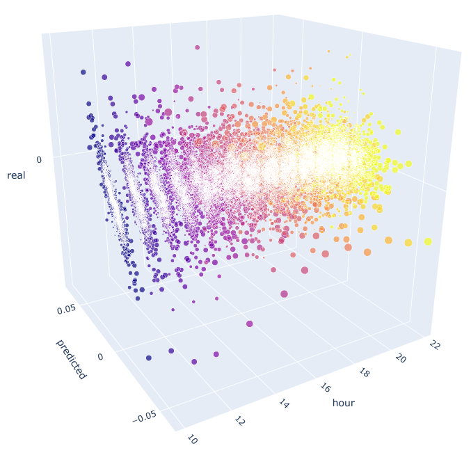
Fig. 10. 3D scatter plot for actual and predicted increments from 2015 to 2020.
Now it's time to create an Expert Advisor to see how it works.
Example of an Expert Advisor trading the identified seasonal patterns
Similarly to an example from the previous article, the robot will trade a seasonal pattern which is only based on the statistical relationship between the current increment and the previous one for one specific hour. The difference is that other hours are traded and a principle based on the proposed formula is used.
Let's consider an example of using the resulting formula for trading, based on the statistical study:
input int OpenThreshold = 30;     //Open threshold
input int OpenThreshold1 = 30;    //Open threshold 1
input int OpenThreshold2 = 30;    //Open threshold 2
input int OpenThreshold3 = 30;    //Open threshold 3
input int OpenThreshold4 = 30;    //Open threshold 4
input int Lag = 10;
input int stoploss = 150;         //Stop loss
input int OrderMagic = 666;       //Orders magic
input double   MaximumRisk=0.01;  //Maximum risk
input double   CustomLot=0;       //Custom lot
The following interval with patterns was determined: {10, 11, 12, 13, 14}. Based on it, the "Open threshold" parameter can be set for each hour individually. These parameters are similar to "rfilter" in fig. 9. The 'Lag' variable contains the lag value for the increments (remember, we analyzed the lag of 25 by default, i.e. almost a day for the H1 timeframe). Lags could be set separately for each hour, but the same value for all hours is used here for simplicity purposes. Stop Loss is also the same for all positions. All these parameters can be optimized.
The trading logic is as follows:
void OnTick() {
//---
   if(!isNewBar()) return;
   CopyClose(NULL, 0, 0, Lag*2+1, prArr);
   ArraySetAsSeries(prArr, true);
   const double pr = (prArr[1] - prArr[Lag]) - ((prArr[Lag] - prArr[Lag*2]) - (prArr[Lag-1] - prArr[Lag*2-1]));

   TimeToStruct(TimeCurrent(), hours);

   if(hours.hour >=10 && hours.hour <=14) {

      //if(countOrders(0)==0)
      //   if(pr >= signal && CheckMoneyForTrade(_Symbol,LotsOptimized(),ORDER_TYPE_BUY))
      //      OrderSend(Symbol(),OP_BUY,LotsOptimized(), Ask,0,Bid-stoploss*_Point,NormalizeDouble(Ask + signal, _Digits),NULL,OrderMagic,INT_MIN);

      if(CheckMoneyForTrade(_Symbol,LotsOptimized(),ORDER_TYPE_SELL)) {
         if(pr <= -signal && hours.hour==10)
            OrderSend(Symbol(),OP_SELL,LotsOptimized(), Bid,0,Ask+stoploss*_Point,NormalizeDouble(Bid - signal, _Digits),NULL,OrderMagic);
         if(pr <= -signal1 && hours.hour==11)
            OrderSend(Symbol(),OP_SELL,LotsOptimized(), Bid,0,Ask+stoploss*_Point,NormalizeDouble(Bid - signal1, _Digits),NULL,OrderMagic);
         if(pr <= -signal2 && hours.hour==12)
            OrderSend(Symbol(),OP_SELL,LotsOptimized(), Bid,0,Ask+stoploss*_Point,NormalizeDouble(Bid - signal2, _Digits),NULL,OrderMagic);
         if(pr <= -signal3 && hours.hour==13)
            OrderSend(Symbol(),OP_SELL,LotsOptimized(), Bid,0,Ask+stoploss*_Point,NormalizeDouble(Bid - signal3, _Digits),NULL,OrderMagic);
         if(pr <= -signal4 && hours.hour==14)
            OrderSend(Symbol(),OP_SELL,LotsOptimized(), Bid,0,Ask+stoploss*_Point,NormalizeDouble(Bid - signal4, _Digits),NULL,OrderMagic);
      }
   }
}
The 'pr' constant is calculated by the above specified formula. This formula forecasts price increment on the next bar. Condition for each hour is checked then. If the increment meets the minimum threshold for the particular hour, a sell deal is opened. We have already found out that shifting the average increments to the negative zone makes purchases ineffective in the interval from 2015 to 2020, you can check it yourself.
Let's launch genetic optimization with parameters specified in fig. 11 and view the result:
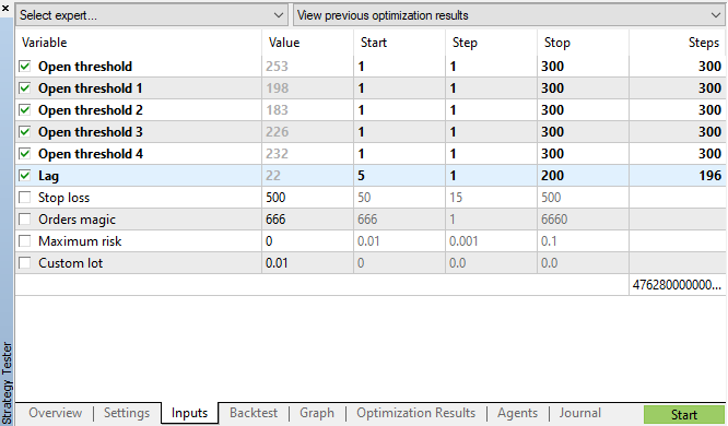
Fig. 11. The table of genetic optimization parameters
Let's look at the optimization chart. In the optimized interval, the most efficient Lag values are located between 17-30 hours, which is very close to our assumption about the dependence of increments of a particular hour on the current day on the same hour of the previous day:
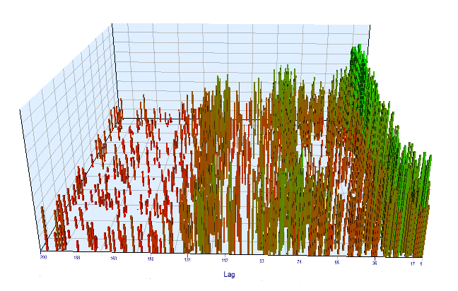
Fig. 12. Relationship of the 'Lag' variable to the 'Order threshold' variable in the optimized interval
The forward chart looks similarly:
Fig. 13. Relationship of the 'Lag' variable to the 'Order threshold' variable in the forward interval
Here are the best results from the backtest and forward optimization tables:
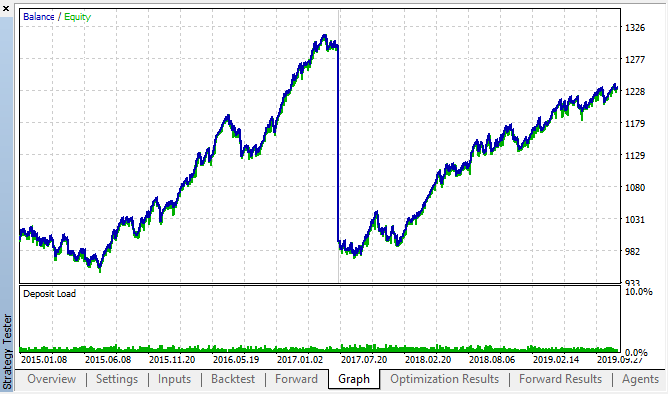
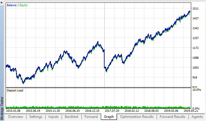
Fig. 14, 15. Backtest and forward optimization charts.
It can be seen that the pattern persists throughout the entire 2015–2020 interval. We can assume that the econometric approach worked perfectly well. There are dependencies between same hour increments for the next days of the week, with some clustering (the dependence may not be with the same hour, but with a nearby hour). In the next article, we will analyze how to use the second pattern.
Check the increment period on another timeframe
Let us perform an additional check on the M15 timeframe. Suppose we are looking for the same correlation between the current hour and the same hour of the previous day. In this case the effective lag must by 4 times larger and be about 24*4 = 96, because each hour contains four M15 periods. I have optimized the Expert Advisor with the same settings and with the M15 timeframe.
In the optimized interval, the resulting effective lag is <60, which is strange. Probably the optimizer found another pattern, or the EA was overoptimized.
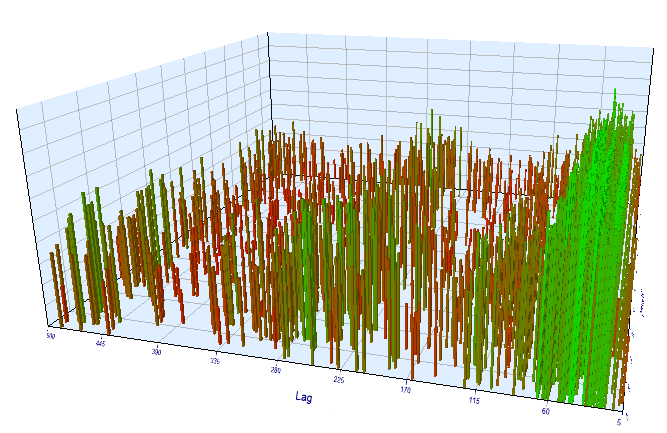
Fig. 16. Relationship of the 'Lag' variable to the 'Order threshold' variable in the optimized interval
As for the forward test results, the effective lag is normal and corresponds to 100, which confirms the pattern.
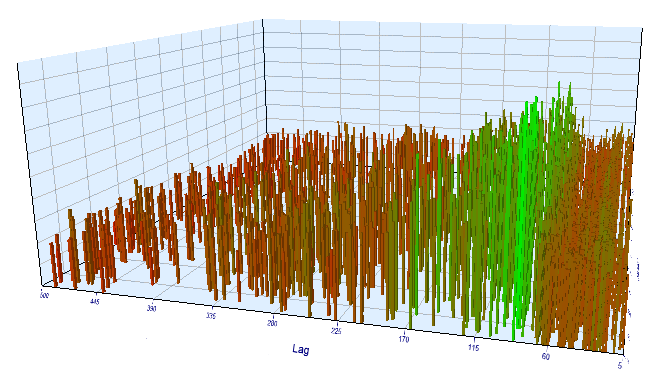
Fig. 17. Relationship of the 'Lag' variable to the 'Order threshold' variable in the forward interval
Let us view the best backtest and forward results:
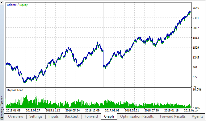
Fig. 18. Backtest and forward; the best forward pass
The resulting curve is similar to the H1 chart curve, with a significant increase in the number of deals. Probably, the strategy can be optimized for lower timeframes.
Conclusion
In this article, we put forward the following hypothesis:
Correlation of price increments depends on the presence of seasonal patterns, as well as on the clustering of nearby increments.
The first part has been fully confirmed: there is correlation between hourly increments form different weeks. The second statement has been implicitly confirmed: the correlation has clustering, which means that current hour increments also depend on the increments of neighboring hours.
Please note that the proposed Expert Advisor is by no means the only possible variant for trading the found correlations. The proposed logic reflects the author’s view on correlations, while the EA optimization was only performed to additionally confirm the patterns found through statistical research.
Since the second part of our study requires additional substantial research, we will use a simple machine learning model in the next article to totally confirm or refute the second part of the hypothesis.
The attachment contains a ready-to-use framework in the Jupyter notebook format, which you can use to study other financial instruments. The results can further be tested using the attached testing EA.