Applying the probability theory to trading gaps
Aleksey Nikolayev | 30 January, 2019
Contents
- Introduction
- General considerations concerning Expert Advisors
- Trading strategy as an attempt to reject the random walk hypothesis
- Gap trading strategy
- Testing the strategy and calculating the optimal risk per deal
- Conclusion
- Attached files
Introduction
The article continues the topic of applying the probability theory and mathematical statistics in trading started in the author's previous articles. We will consider possible use of the appropriate methods for creating and testing trading strategies.
First, we will look at finding such trading possibilities as detecting deviations from the random walk hypothesis. It is proved that if prices behave like a zero-drift random walk (with no directional trend), then profitable trading is impossible. This provides a basis for finding ways to refute this hypothesis. If a way to refuting the hypothesis is found, we may try to use that to develop a trading strategy.
We will also continue studying the topic of risk we started in the previously published articles. Further on, we will refer to them as the first and second articles.
Since our approach is based on the probability theory, understanding of its foundations is advisable but not mandatory. It is important to understand the essence of probabilistic methods − the more systematically and often they are used, the more noticeable and significant the result obtained (due to the law of large numbers). Of course, their application should be sufficiently substantiated and adequate.
General considerations concerning Expert Advisors
Developing EAs can be roughly divided into three stages:
- Generating an idea.
- Checking the idea using all sorts of simplifications.
- Adapting the idea to the market realities.
The article will mainly deal with the second stage allowing us to focus on the stated topic more thoroughly. Besides, this stage is discussed on the forum much less frequently than the others.
Let's describe the implemented simplifications. We will confine ourselves to EAs trading a single asset. We will assume that the asset price is expressed in the account currency. We will exclude non-trading operations (like swap and withdrawing funds from the account) and will not consider different types of orders (leaving only buying and selling by market prices). We will neglect slippage when executing orders, while spread (s) is to be considered a fixed value. We will also assume that the EA manages all the funds on our account, and there are no other EAs launched on it.
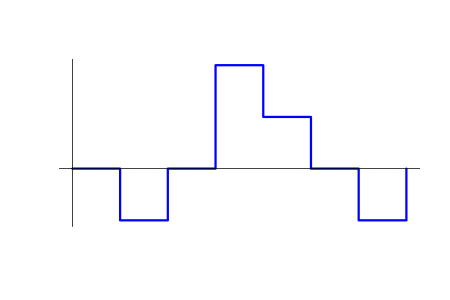
With all these simplifications, the EA operation result is unambiguously defined as the v(t) function − position volume depending on time. Positive v(t) corresponds to buying, while negative one means selling. Besides, there is the p(t) (asset price) function and c0 (initial funds). The image below shows the possible v=v(t) position chart.
The arithmetic average between buy and sell prices.
The v(t) and p(t) are piecewise constant (stepwise) functions since their values are multiples of some minimal increment steps. If a more rigorous mathematical definition is needed, then they can be considered continuous from the right and having a limit at the gap points on the left. We assume that the v(t) gap points never match the p(t) ones. In other words, no more than one value from the two can change at any moment in time − either a price, or a position volume, or both remain unchanged. It is worth noting that the points in time, at which price or volume changes may occur, are also multiples of a certain minimum step.
Based on these data, we can find the c (t) function − the value of funds depending on time. It is defined as the balance value for the part of the account managed by the EA in case we would close a position at the t moment. Since we have a single EA on the account, this value coincides with the account equity defined in MetaTrader 5.
Define c(t) change at t. If the volume and price do not change at this moment, then it is naturally zero. If the price changes, the funds increase is equal to the product of the volume by the price increment. If the volume changes, two options are possible − when the absolute position volume is decreased, the funds remain the same, when it is increased, the funds are decreased by an amount equal to the product of the spread by the absolute value of the volume change. In other words, if a position is closed partially, the equity does not change, while adding to the position leads to the equity slight decrease. Thus, c(t) funds value at the t moment is equal to the sum of c0=c(0) and all of its changes that occurred from the zero moment up to t.
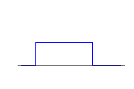
When developing our risk theory (in the two previous articles), we used the concept of a 'deal'. This concept does not quite coincide with what is called a 'deal' in MetaTrader 5 and more corresponds to what is called a 'trade' there. To be exact, it corresponds to what we call a simple position. A simple position, by our definition, is set by the moments of opening and closing. Its volume and direction remain constant between that moments. Below is a sample v=v(t) chart for a simple position.
Any position (since it is always piecewise constant) can be imagined as a sum of simple positions. Such a representation can be done in an infinite number of ways. The chart below shows a single position represented in two different ways as a sum of simple ones. The initial position is shown in blue, while deals it is divided into are displayed in green and red. When using a concept of trades in MetaTrader 5, we get yet another option. Each of these methods can be quite reasonable.

There are some EAs, for which such representations do not make much sense. For example, there may be EAs where a position is gradually increased and is gradually decreased afterwards. At the same time, there are EAs, for which such a presentation is quite natural. For example, a position may consist of a sequence of simple positions that do not intersect in time. The chart below contains examples of such positions.

Relative change of funds c1/c0 after each deal (simple position) is expressed in two values − profitability a and risk r: c1/c0=1+ra. The profitability is equal to the ratio of the price increase during the deal to the difference between entry prices and stop loss, while the risk is proportional to the deal volume and means a share of funds that would be lost in case of stop loss exact activation.
Thus, instead of considering the v(t), p(t) and c(t) time functions, we turn to analyzing numerical sequences characterizing the sequence of deals. This greatly simplifies further study. In particular, we avoid the need to apply the theory of random processes limiting ourselves to finite sets of random variables when proceeding to the probabilistic model of uncertainty.
The probability theory is a generally accepted method of mathematical modeling of uncertainty in the behavior of asset prices and in trading results. In accordance with this approach, we should consider the v(t), p(t) and c(t) functions as specific implementations (trajectories) of some random processes. In general terms, this task is practically unsolvable. The main reason is the lack of adequate probabilistic models accurately describing the price behavior. Therefore, it makes sense to consider special cases where a solution is possible. As mentioned above, in this article, we will consider EAs forming positions that can be adequately represented as a sequence of simple positions (deals).
It is worth mentioning another issue related to EAs – parameters. It would be useful to consider them in details to achieve some formalization (standardization) of the EA development process. Let's divide the parameters into three types:
- Historical parameters. Parameters that may change during the EA operation from one deal to another. These are indicator values, time of day, news data, moon phases, etc. In general, they are time functions, just like prices or position volumes. In case of applied simplification, we can consider them to be sequences of numbers known at the moment of making a deal. Parameters of each specific deal (direction, volume, stop loss and take profit) are defined based on the values of historical parameters.
- Actual parameters. Let's simply call them the parameters for brevity. They are set when an EA starts trading and can be applied only when testing and optimizing the EA.
- Meta-parameters set the EA optimization algorithm, for example, custom optimization criterion parameter. Suppose that we want to optimize the EA by two criteria, although this can be done only by one. We form a new criterion of the two original ones taking their sum with some weights. These weights are served as meta-parameters.
For example, in the gap-based EA described below, the minimum gap is the EA parameter, while the size of each specific gap is a historical parameter. In this case, meta parameters may include optimization criterion number (we assume that the criteria are numbered in some order, for example, optimization by profit is #1, while optimization by drawdown is #2, etc.).
In this article, we will use one significant simplification associated with historical parameters. When we talk about the distribution of returns in a deal, it may generally depend on these parameters. We assume this dependence is insignificant. The main reason is that an attempt to take into account this dependence usually over-complicates the model, which may eventually lead to an over-fitting.
Trading strategy as an attempt to reject the random walk hypothesis
We have already mentioned the absence of accurate models describing the price behavior. Nevertheless, there are approximate models that can be useful. For example, there is a well-known price behavior model considering prices to be a random walk with a zero drift (absence of a directed trend). This model is called the random walk hypothesis. According to this hypothesis, any EA will have a zero profit on average or a small loss if we take a spread into account.
Proving the impossibility of making money on a random walk is rather difficult because it requires the involvement of a complex mathematical apparatus of the theory of random processes (Itô calculus, Stopping time, etc). In general, it boils down to the statement that when trading on a random walk without a trend, the capital is a martingale (probability theory, not to be confused with martingale as a betting system). A martingale is a random process with its average value (mathematical expectation) not changing with time. In our case, this means that the mathematical expectation of the value of capital at any time is equal to its initial value.
Thus, we should start our consideration of a trading idea from searching for statistically significant price deviations from the random walk. To do this, we will use ideas from the probability theory and mathematical statistics, but first, let's make a few observations:
- Any solution of this kind is probabilistic in nature − there is always some non-zero probability that our conclusions are wrong.
- If our method does not detect deviations, this does not mean their complete absence. Perhaps, some other method would detect them.
- Statistically significant deviations do not guarantee obtaining statistically significant positive profits − the presence of deviations is necessary but not a sufficient condition for this.
Let's construct a method to search for random walk deviations. To do this, we will consider some random variable, for which we will build an empirical probability distribution based on a sample formed using real prices. Besides, we will construct a theoretical probability distribution for the same value assuming that the price behavior is a random walk. Comparing these distributions, we will make a decision about rejecting (or impossibility to reject) the random walk hypothesis.
Let's construct an example of a suitable value. Suppose that at the t0 initial moment in time, the price is equal to p0. Let's take another p1 price value not equal to p0. Wait till t1 moment when the price reaches that value p(t1)=p1. Let's find the price p2 which is the farthest one from p1 out of the prices in the time interval between t0 and t1. Let's introduce the value K=(p2-p0)/(p0-p1). The p1<p0≤p2 or p2≤p0<p1 condition is always in effect, therefore K≥0 at all times. The chart explaining this idea is provided below. The blue line means p0 price level, while the moment it crosses the price chart is t0. The red line means p1 price level, while the moment it touches the price chart after t0 is t1. The green line means the p2 price level located as far from p1 as possible.
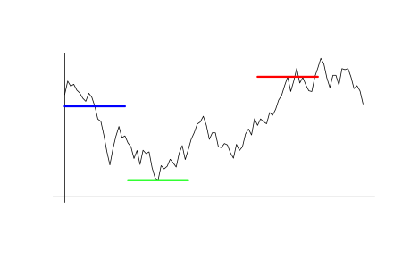
The idea behind the value is simple. Suppose that we enter a deal at t0. Let it be selling at p0, while p1, p1>p0 − stop loss. p2 is the least achievable price for a take profit, while K is the highest achievable profit for a deal. In reality, we do not know the exact K value when performing a transaction. Within the framework of the probabilistic model of this uncertainty, we can only talk about knowing its probability distribution pattern. Suppose that we know the Fk(x) probability distribution function, which is defined as the probability that K<x. Suppose that we use a certain pk price as a take profit: pk-p0=k(p0-p1). In this case, Fk(k) is equal to the probability that a stop loss is reached earlier than take profit. Accordingly, 1-Fk(k) is equal to the probability that the take profit is activated earlier. Let the spread be equal to zero for now. Then, in case of stop loss activation, the profitability is equal to -1, while in case of take profit activation, it is equal to k. The mathematical expectation in such a deal: M=(-1)*Fk(k)+k*(1-Fk(k))=k-(k+1)*Fk(k), which is equal to zero if Fk(k)=k/(k+1).
If we know the equation form Fk(x), we even can perform a preliminary optimization of an EA. For example, we can look for the optimal take profit/stop loss ratio that maximizes the mathematical expectation of the deal's profitability. Then we can find the optimal risk value in the deal. Thus, the EA can be optimized even before it is ready. This saves time and allows you to discard obviously unsuitable ideas at an early stage.
If we assume that prices behave like a random walk without a trend, then the distribution of the K value is set by the Fk(x)=Fk0(x) distribution function, where Fk0(x)=0 if x≤0 and Fk0(x)=x/(x+1) if x>0. For more certainty, we can assume that the random walk used here is a Wiener process with zero drift (no trend). As we can see, if the random walk hypothesis is fulfilled and the spread is equal to zero, the mathematical expectation of the profitability is equal to zero at any take profit/stop loss ratio. In case of a non-zero spread, it is negative.
Instead of K, we can consider the value Q=K/(K+1)=(p2-p0)/(p2-p1), K=Q/(1-Q). This value can be represented as the ratio of take profit to the sum of stop loss and take profit. It is more convenient because it takes values within the [0;1) interval and has a simpler distribution than K (uniform on this interval) in case of a random walk.
Further on, we will talk mainly about the Q value. Let's consider how its empiric distribution function Fq(x) is constructed and applied. Suppose that we have a trading idea we check on price history. We have a set of n entry points. The entry price p0,i and stop loss p1,i, where i=1,...,n, is defined for each of them. Now we should define if this idea has some profit potential. For each deal, we should find the price p2,i located as far as possible from the stop loss till the moment of its activation. Based on the prices, we get the n sample Qi=(p2,i-p0,i)/(p2,i-p1,i), i=1,...,n. The empirical distribution function constructed by this sample is defined by the Fq(x)=m(x)/n equation where m(x) is equal to the number of Qi sample elements smaller than x. If prices behave like a random walk without a trend (Wiener process with zero drift), the Fq0(x) distribution function of the Q value looks simple: Fq0(x)=0 if x≤0, Fq0(x)=x if 0<x≤1, and Fq0(x)=1 if x>1.
If Fq(x) is significantly different from the theoretical distribution function with a random walk Fq0(x), we need to check the significance of this difference in terms of profitability. If the profitability is sufficiently positive even if the spread is taken into account, then it is time to choose the appropriate profit/stop loss ratio. This can be done by maximizing the profitability expectation. After that, we can select an optimal value for the risk value per deal and move on to preliminarily test the idea. If the result is positive, it makes sense to proceed to the creation of an actual trading EA. Further on, we will try to show this algorithm in real practice.
The question arises – how to make similar comparisons with a random walk for more complex market exit algorithms. The general answer is in the same way as for the case considered above. The main issue is that the distribution of profitabilities on a random walk can be obtained in an analytical form in quite rare occasions. But it is always possible to get its empirical approximation using the Monte Carlo simulation method.
Gap trading strategy
Before analyzing the idea, I should note that our main task is to demonstrate the analysis methods, not profitable trading strategies. Too much concentration on profit would have buried us under trifle details distracting us from the overall picture.
Asset prices are discrete and therefore always change in leaps and bounds. These leaps may differ in size. When they are large, they are called gaps. There is no certain boundary separating gaps from usual price changes. We are free to set that boundary where we see fit.
Gaps are well suited for demonstrating the theory outlined in the previous section. Each of them is set by two time points and asset prices within them. Using the previously introduced price notation, we assume that p0 is a later price, while p1 is an earlier one. We enter a trade as soon as a gap occurs. The price p1 can be considered not only as a stop loss, but also as a take profit. This means that we can choose a system of one of two types − hoping either for a quick closure of the gap, or for a large price movement in the direction of the gap. The gap closure means the price returns to the p1 level or breaks it through.
Since gaps in their standard form are relatively rare for Forex assets, the author was offered to generalize this concept when discussing the topic of this article with the forum administration. When defining a gap, you may abandon the requirement stating that only a gap between two subsequent prices is taken into account. Obviously, the number of possible gaps in this case will become unimaginably huge and therefore it is worthwhile to limit ourselves by the options reasonable from a trading point of view. For example, the author was offered to consider gaps between the closing price of one American session and the opening price of the next one.
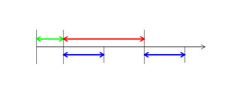
Let me explain how the concept of a session is formalized. It is set by the three time intervals: period, length and shift. Sessions are periodic and have a length that does not exceed the period. Any tick either belongs to any session or does not belong to any of them (the latter is possible if its length is strictly less than the period). The shift is a time interval between the zero point in time and the beginning of the first session after it. It should be less than the period. This concept of the session is somewhat wider than usual and allows us to consider, for example, gaps between the minute bars. Let's illustrate it in the diagram below. The green arrow represents the length of time defining the shift, the red one shows the period, while the blue one demonstrates the session length.
We will use two slightly different EAs to collect statistics related to gaps. The first one (gaps_reg_stat.mq5) considers gaps between the two subsequent ticks, while the second one (gaps_ses_stat.mq5) considers gaps between sessions. Of course, these EAs do not trade and run only in test mode. It is recommended to run the first of them only on real ticks, while the second one − on OHLC of minute bars. The EA codes are provided below.
// gaps_reg_stat.mq5
#define ND 100

input double gmin=0.1;                 // minimal gap size: USDJPY - 0.1, EURUSD - 0.001
input string fname="gaps\\stat.txt";   // name of file for statistics

struct SGap
  { double p0;
    double p1;
    double p2;
    double p3;
    double s;
    void set(double p_1,double p,double sprd);
    bool brkn();
    void change(double p);
    double gap();
    double Q();
  };

class CGaps
  { SGap gs[];
    int ngs;
    int go[];
    int ngo;
    public:
    void init();
    void add(double p_1,double p,double sprd);
    void change(double p);
    void gs2f(string fn);
  };

CGaps gaps;
MqlTick tick0;
bool is0=false;

void OnTick()
  { MqlTick tick;
    if (!SymbolInfoTick(_Symbol, tick)) return;
    if(is0)
      { double p=(tick.bid+tick.ask)*0.5, p0=(tick0.bid+tick0.ask)*0.5;
        gaps.change(p);
        if(MathAbs(p-p0)>=gmin) gaps.add(p0,p,tick.ask-tick.bid);
      }
    else is0=true;
    tick0=tick;
  }

int OnInit()
  { gaps.init();
     return(INIT_SUCCEEDED);
  }

void OnDeinit(const int reason)
  { gaps.gs2f(fname);
  }

void SGap :: set(double p_1,double p,double sprd)
  { p1=p_1; p0=p2=p3=p; s=sprd;
  }

bool SGap :: brkn()
  { return ((p0>p1)&&(p3<=p1))||((p0<p1)&&(p3>=p1));
  }

void SGap :: change(double p)
  { if(brkn()) return;
    if((p0>p1&&p>p2) || (p0<p1&&p<p2)) p2=p;
    p3=p;
  }

double SGap :: gap()
  { return MathAbs(p0-p1);
  }

double SGap :: Q()
  { double q=p2-p1;
    if(q==0.0) return 0.0;
    return (p2-p0)/q;
  }

void CGaps :: init()
  { ngs=ngo=0;
  }

void CGaps :: add(double p_1,double p,double sprd)
  { ++ngs;
    if(ArraySize(gs)<ngs) ArrayResize(gs,ngs,ND);
    gs[ngs-1].set(p_1,p,sprd);
    int i=0;
    for(; i<ngo; ++i) if(go[i]<0) break;
    if(i==ngo)
      {
        ++ngo;
        if(ArraySize(go)<ngo) ArrayResize(go,ngo,ND);
      }
    go[i]=ngs-1;
  }

void CGaps :: change(double p)
  { for(int i=0; i<ngo; ++i)
      { if(go[i]<0) continue;
        gs[go[i]].change(p);
        if(gs[go[i]].brkn()) go[i]=-1;
      }
  }

void CGaps :: gs2f(string fn)
  { int f=FileOpen(fn, FILE_WRITE|FILE_COMMON|FILE_ANSI|FILE_TXT), c;
    for(int i=0;i<ngs;++i)
      { if (gs[i].brkn()) c=1; else c=0;
        FileWriteString(f,(string)gs[i].gap()+" "+(string)gs[i].Q()+" "+(string)c+" "+(string)gs[i].s);
        if(i==ngs-1) break;
        FileWriteString(f,"\n");
      }
    FileClose(f);
  }
// gaps_ses_stat.mq5
#define ND 100

input double gmin=0.001;               // minimal gap size: USDJPY - 0.1, EURUSD - 0.001
input uint   mperiod=1;                // session period in minutes
input uint   mlength=1;                // session length in minutes
input uint   mbias=0;                  // first session bias in minutes
input string fname="gaps\\stat.txt";   // name of file for statistics

struct SGap
  { double p0;
    double p1;
    double p2;
    double p3;
    double s;
    void set(double p_1,double p,double sprd);
    bool brkn();
    void change(double p);
    double gap();
    double Q();
  };

class CGaps
  { SGap gs[];
    int ngs;
    int go[];
    int ngo;
    public:
    void init();
    void add(double p_1,double p,double sprd);
    bool change(double p);
    void gs2f(string fn);
  };

CGaps gaps;
MqlTick tick0;
int ns0=-1;
ulong sbias=mbias*60, speriod=mperiod*60, slength=mlength*60;

void OnTick()
  { MqlTick tick;
    if (!SymbolInfoTick(_Symbol, tick)) return;
    double p=(tick.bid+tick.ask)*0.5;
    gaps.change(p);
    int ns=nsession(tick.time);
    if(ns>=0)
      { double p0=(tick0.bid+tick0.ask)*0.5;
        if(ns0>=0&&ns>ns0&&MathAbs(p-p0)>=gmin) gaps.add(p0,p,tick.ask-tick.bid);
        ns0=ns;
        tick0=tick;
      }
  }

int OnInit()
  { if(speriod==0||slength==0||speriod<slength||speriod<=sbias)
      { Print("wrong session format");
        return(INIT_FAILED);
      }
    gaps.init();
    return(INIT_SUCCEEDED);
  }

void OnDeinit(const int reason)
  { gaps.gs2f(fname);
  }

int nsession(datetime t)
  { ulong t0=(ulong)t;
    if(t0<sbias) return -1;
    t0-=sbias;
    if(t0%speriod>slength) return -1;
    return (int)(t0/speriod);
  }

void SGap :: set(double p_1,double p,double sprd)
  { p1=p_1; p0=p2=p3=p; s=sprd;
  }

bool SGap :: brkn()
  { return ((p0>p1)&&(p3<=p1))||((p0<p1)&&(p3>=p1));
  }

void SGap :: change(double p)
  { if(brkn()) return;
    if((p0>p1&&p>p2) || (p0<p1&&p<p2)) p2=p;
    p3=p;
  }

double SGap :: gap()
  { return MathAbs(p0-p1);
  }

double SGap :: Q()
  { double q=p2-p1;
    if(q==0.0) return 0.0;
    return (p2-p0)/q;
  }

void CGaps :: init()
  { ngs=ngo=0;
  }

void CGaps :: add(double p_1,double p,double sprd)
  { ++ngs;
    if(ArraySize(gs)<ngs) ArrayResize(gs,ngs,ND);
    gs[ngs-1].set(p_1,p,sprd);
    int i=0;
    for(; i<ngo; ++i) if(go[i]<0) break;
    if(i==ngo)
      {
        ++ngo;
        if(ArraySize(go)<ngo) ArrayResize(go,ngo,ND);
      }
    go[i]=ngs-1;
  }

bool CGaps :: change(double p)
  { bool chngd=false;
    for(int i=0; i<ngo; ++i)
      { if(go[i]<0) continue;
        gs[go[i]].change(p);
        if(gs[go[i]].brkn()) {go[i]=-1; chngd=true;}
      }
    return chngd;
  }

void CGaps :: gs2f(string fn)
  { int f=FileOpen(fn, FILE_WRITE|FILE_COMMON|FILE_ANSI|FILE_TXT), c;
    for(int i=0;i<ngs;++i)
      { if (gs[i].brkn()) c=1; else c=0;
        FileWriteString(f,(string)gs[i].gap()+" "+(string)gs[i].Q()+" "+(string)c+" "+(string)gs[i].s);
        if(i==ngs-1) break;
        FileWriteString(f,"\n");
      }
    FileClose(f);
  }
The EAs are quite simple, although it makes sense to mention the go[] array in the CGaps class where the indices of unclosed gaps are stored allowing to speed up the EAs' work.
In any case, the following data is recorded for each gap: absolute gap value, Q value, data on its closure and spread value at the moment of the gap. Then, the difference between the Q empiric distribution value and the uniform one is checked and the decision on further analysis is made. Graphical and computational (Kolmogorov statistics calculation) methods are used to check the difference. For simplicity, we will restrict ourselves to the p-value of the Kolmogorov-Smirnov test as a result of calculations. It takes values between zero and one, and the smaller it is, the less likely it is that the distribution of the sample coincides with the theoretical one.
We selected the Kolmogorov-Smirnov (one-sample) test for mathematical considerations. The main reason is that we are interested in distinguishing the distribution functions in the uniform convergence metric, not in any integral metrics. This test was not found in the MQL5 libraries, so I had to use the R language. It is worth noting that if there are matching numbers in the sample, the accuracy of this criterion is somewhat reduced (R gives an appropriate warning) but remains quite acceptable.
If a significant discrepancy between the theoretical and empirical distributions are discovered, we should study the possibility of extracting profit from that. If there is no significant discrepancy, then we either discard this idea or try to improve it.
As I mentioned above, there are two ways to enter a transaction at the p0 price when a gap is formed − either in the gap direction or in the opposite one. Let's calculate the expectation of returns for both these cases. While doing that, we will consider a spread considering it to be constant and denoting it as s. The absolute gap value is denoted as g, while g0 stands for its minimum value.
- Entry in the gap direction. In this case, g+s is a stop loss, while kg-s is a take profit. Here k is a profit/loss ratio. Profitability values: -1 in case of a stop loss activation and (kg-s)/(g+s) in case of a take profit activation. Corresponding probabilities: Fq(q) and 1-Fq(q). Let's express k via q: k=k(q)=q/(1-q). Then for the mathematical expectation of profitability M, M=Fq(q)*(-1)+(1-Fq(q))*(k(q)g-s)/(g+s). Only the q values, for which M is significantly positive for all g≥g0, are suitable for us. We will need the q values, at which Fq(q) is significantly lower than the theoretical value with the random walk Fq(q)<Fq0(q) at g=g0.
- Counter-gap entry. In this case, g-s is a take profit, while kg+s is a stop loss. Here k is a loss/profit ratio. Profitability values: -1 in case of a stop loss activation and (g-s)/(kg+s) in case of a take profit activation. Corresponding probabilities: 1-Fq(q) and Fq(q). The expression for k via q is the same as in the previous passage: k=k(q)=q/(1-q). For profitability mathematical expectation M, we obtain the equation M=(1-Fq(q))*(-1)+*Fq(q)(g-s)/(k(q)g+s). Only the q values, for which M is significantly positive for all g≥g0, are suitable for us. We will need the q values, at which Fq(q) is significantly higher than the theoretical value Fq(q)>Fq0(q) at g=g0.
Statistics were collected for two symbols:
- EURUSD
- USDJPY
The following types of gaps were considered for each of them:
- Between consecutive ticks.
- Between minute bars.
- Between trading sessions. For EURUSD, this is an American session (the Chicago and New York ones combined), while for USDJPY, this is a Tokyo one.
For each of these six options, statistics were studied for the most recent:
- 200 gaps
- 50 gaps
As a result, we have 12 options. The results for each of them are as follows:
- p-value for Kolmogorov statistics
- The mean spread value at the moment the gap is formed
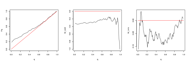
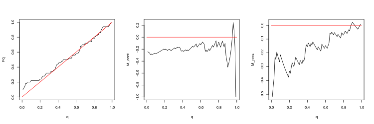
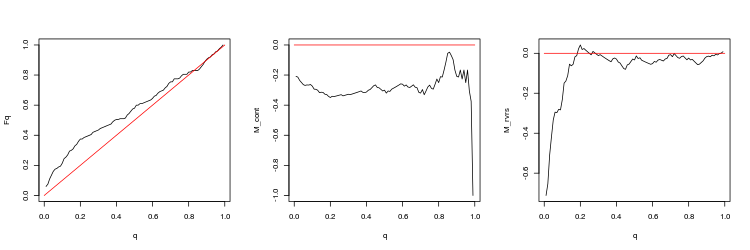
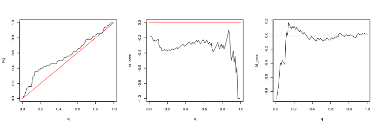
- Graph of the empirical and theoretical (red line) functions of the Q value distribution
- M_cont profitability mathematical expectation graph for trading in a gap direction depending on q as compared to the M_cont=0 theoretical line (red). Here, q means take profit/take profit and stop loss sum ratio.
- M_rvrs profitability mathematical expectation graph for trading opposite to a graph depending on q as compared to the M_rvrs=0 theoretical line (red). Here, q means stop loss/take profit and stop loss sum ratio.
All result options are provided below.
- EURUSD, 200 last gaps between consecutive ticks. p-value: 3.471654e-07, mean spread: 0.000695
- EURUSD, 50 last gaps between consecutive ticks. p-value: 0.2428457, mean spread: 0.0005724
- EURUSD, 200 last gaps between minute bars. p-value: 8.675995e-06, mean spread: 0.0004352
- EURUSD, 50 last gaps between minute bars. p-value: 0.0125578, mean spread: 0.000404
- EURUSD, 200 last gaps between trading sessions. p-value: 0.6659917, mean spread: 0.0001323
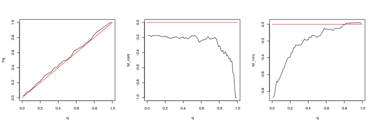
- EURUSD, 50 last gaps between trading sessions. p-value: 0.08915716, mean spread: 0.0001282
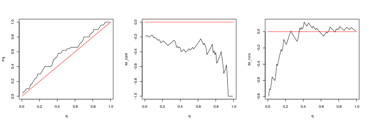
- USDJPY, 200 last gaps between consecutive ticks. p-value: 2.267454e-06, mean spread: 0.09563
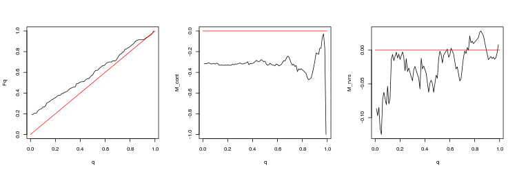
- USDJPY, 50 last gaps between consecutive ticks. p-value: 0.03259067, mean spread: 0.0597
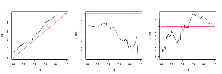
- USDJPY, 200 last gaps between minute bars. p-value: 0.0003737335, mean spread: 0.05148
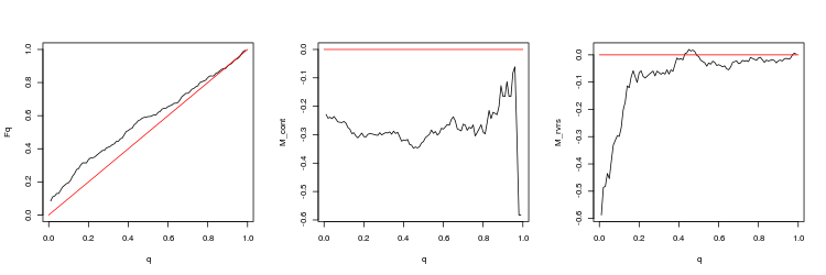
- USDJPY, 50 last gaps between minute bars. p-value: 0.005747542, mean spread: 0.0474
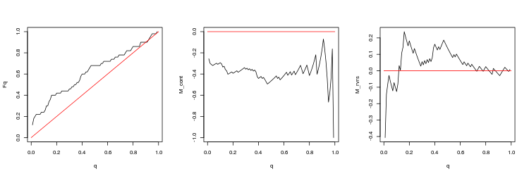
- USDJPY, 200 last gaps between trading sessions. p-value: 0.07743524, mean spread: 0.02023
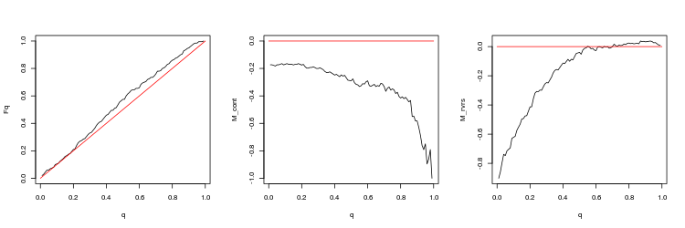
- USDJPY, 50 last gaps between trading sessions. p-value: 0.009191665, mean spread: 0.0185
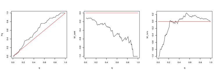
We can draw the following conclusions from these results:
- Deviations from a random walk are quite significant.
- Trading in the gap direction is unpromising. Trading towards the gap closure looks more preferable but the profit is small (especially on EURUSD).
- At the time of gap formation, spreads can grow several times compared with their average value (true for gaps between ticks and minute bars).
- Gaps between trading sessions provide a deviation from a random walk only at some intervals of 1-2 months long, while on year intervals, the deviation is very small. At first glance, this is determined by the trend that is prevalent at a certain time. Apparently, gaps close better during flats and worse during trends, although a more detailed analysis is needed.
- For further analysis, we should choose the gap between minute bars for USDJPY.
Testing the strategy and calculating the optimal risk per deal
The version of the system based on gaps between USDJPY minute bars looks most promising. The significant surge of the spread we have detected at the time of the gap formation means we should pay closer attention to its definition. Let's specify it as follows. We will consider the gap not for the average price, but for the bid and ask. Besides, we will choose the one of them, for which we need to enter the trade. This means, we will define an upward gap by bid and a downward gap — by ask. The same goes for their closure.
Let's develop the EA by slightly changing the one we used for collecting statistics on gaps between sessions. The main change concerns the gap structure. Since we have a definite correspondence between gaps and deals, the entire information necessary for trading (deal volume and closure condition) are to be stored in this structure. Two functions are added for trading. One of them (pp2v()) calculates the volume for each individual deal, while another one (trade()) saves the correspondence between the sum of deal volumes and trading position volume. The EA code (gaps_ses_test.mq5) is provided below.
// gaps_ses_test.mq5
#define ND 100

input uint   mperiod=1;                 // session period in minutes
input uint   mlength=1;                 // session length in minutes
input uint   mbias=0;                   // first session bias in minutes
input double g0=0.1;                    // minimal gap size: USDJPY - 0.1, EURUSD - 0.001
input double q0=0.4;                    // q0=sl/(sl+tp)
input double r=0.01;                    // risk in deal
input double s=0.02;                    // approximate spread
input string fname="gaps\\stat.txt";    // name of file for statistics

struct SGap
  { double p0;
    double p1;
    double p2;
    double v;
    int brkn();
    bool up();
    void change(double p);
    double gap();
    double Q();
    double a();
  };

class CGaps
  { SGap gs[];
    int ngs;
    int go[];
    int ngo;
    public:
    void init();
    void add(double p_1,double p);
    bool change(double pbid,double pask);
    double v();
    void gs2f(string fn);
  };

CGaps gaps;
MqlTick tick0;
int ns0=-1;
ulong sbias=mbias*60, speriod=mperiod*60, slength=mlength*60;
double dv=SymbolInfoDouble(_Symbol,SYMBOL_VOLUME_STEP);

void OnTick()
  { MqlTick tick;
    if (!SymbolInfoTick(_Symbol, tick)) return;
    bool chngd=gaps.change(tick.bid,tick.ask);
    int ns=nsession(tick.time);
    if(ns>=0)
      { if(ns0>=0&&ns>ns0)
          { if(tick0.ask-tick.ask>=g0) {gaps.add(tick0.ask,tick.ask); chngd=true;}
              else if(tick.bid-tick0.bid>=g0) {gaps.add(tick0.bid,tick.bid); chngd=true;}
          }
        ns0=ns;
        tick0=tick;
      }

    if(chngd) trade(gaps.v());
  }

int OnInit()
  {
     gaps.init();
     return(INIT_SUCCEEDED);
  }

void OnDeinit(const int reason)
  { gaps.gs2f(fname);
  }

int nsession(datetime t)
  { ulong t0=(ulong)t;
    if(t0<sbias) return -1;
    t0-=sbias;
    if(t0%speriod>slength) return -1;
    return (int)(t0/speriod);
  }

double pp2v(double psl, double pen)
  { if(psl==pen) return 0.0;
    double dc, dir=1.0;
    double c0=AccountInfoDouble(ACCOUNT_EQUITY);
    bool ner=true;
    if (psl<pen) ner=OrderCalcProfit(ORDER_TYPE_BUY,_Symbol,dv,pen+s,psl,dc);
      else {ner=OrderCalcProfit(ORDER_TYPE_SELL,_Symbol,dv,pen,psl+s,dc); dir=-1.0;}
    if(!ner) return 0.0;
    return -dir*r*dv*c0/dc;
  }

void trade(double vt)
  { double v0=SymbolInfoDouble(_Symbol,SYMBOL_VOLUME_MIN);
    if(-v0<vt<v0) vt=v0*MathRound(vt/v0);
    double vr=0.0;
    if(PositionSelect(_Symbol))
      { vr=PositionGetDouble(POSITION_VOLUME);
        if(PositionGetInteger(POSITION_TYPE)==POSITION_TYPE_SELL) vr=-vr;
      }
    int vi=(int)((vt-vr)/dv);
    if(vi==0) return;
    MqlTradeRequest request={0};
    MqlTradeResult  result={0};
    request.action=TRADE_ACTION_DEAL;
    request.symbol=_Symbol;
    if(vi>0)
      { request.volume=vi*dv;
        request.type=ORDER_TYPE_BUY;
      }
      else
        { request.volume=-vi*dv;
          request.type=ORDER_TYPE_SELL;
        }
    if(!OrderSend(request,result)) PrintFormat("OrderSend error %d",GetLastError());
  }

int SGap :: brkn()
  { if(((p0>p1)&&(p2<=p1))||((p0<p1)&&(p2>=p1))) return 1;
    if(Q()>=q0) return -1;
    return 0;
  }

bool SGap :: up()
  { return p0>p1;
  }

void SGap :: change(double p)
  { if(brkn()==0) p2=p;
  }

double SGap :: gap()
  { return MathAbs(p0-p1);
  }

double SGap :: Q()
  { if(p2==p1) return 0.0;
    return (p2-p0)/(p2-p1);
  }

double SGap :: a()
  { double g=gap(), k0=q0/(1-q0);
    return (g-s)/(k0*g+s);
  }

void CGaps :: init()
  { ngs=ngo=0;
  }

void CGaps :: add(double p_1,double p)
  { ++ngs;
    if(ArraySize(gs)<ngs) ArrayResize(gs,ngs,ND);
    gs[ngs-1].p0=gs[ngs-1].p2=p;
    gs[ngs-1].p1=p_1;
    double ps=p+(p-p_1)*q0/(1-q0);
    gs[ngs-1].v=pp2v(ps,p);
    int i=0;
    for(; i<ngo; ++i) if(go[i]<0) break;
    if(i==ngo)
      {
        ++ngo;
        if(ArraySize(go)<ngo) ArrayResize(go,ngo,ND);
      }
    go[i]=ngs-1;
  }

bool CGaps :: change(double pbid,double pask)
  { bool ch=false;
    for(int i=0; i<ngo; ++i)
      { if(go[i]<0) continue;
        if(gs[go[i]].up()) gs[go[i]].change(pbid); else gs[go[i]].change(pask);
        if(gs[go[i]].brkn()!=0) {go[i]=-1; ch=true;}
      }
    return ch;
  }

double CGaps :: v(void)
  { double v=0;
    for(int i=0; i<ngo; ++i) if(go[i]>=0) v+=gs[go[i]].v;
    return v;
  }

void CGaps :: gs2f(string fn)
  { int f=FileOpen(fn, FILE_WRITE|FILE_COMMON|FILE_ANSI|FILE_TXT);
    int na=0, np=0, bk;
    double kt=0.0, pk=0.0;
    for(int i=0;i<ngs;++i)
      { bk=gs[i].brkn();
        if(bk==0) continue;
        ++na; if(bk>0) ++np;
        kt+=gs[i].a();
      }
     if(na>0)
       { kt/=na;
         pk=((double)np)/na;
       }
     FileWriteString(f,"na = "+(string)na+"\n");
     FileWriteString(f,"kt = "+(string)kt+"\n");
     FileWriteString(f,"pk = "+(string)pk);
     FileClose(f);
  }
Let's test the EA on the year of 2017 and define the risk value for trading in 2018 based on its results. The balance/equity graph based on test results of 2017 is provided below.
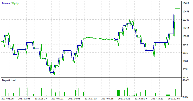
I have to make a few clarifications before proceeding to the risk calculation. First, we need to justify the need to determine the correct level of risk. Second, it is necessary to explain the advantage of applying our theory for this purpose.
Speculative trading is always associated with uncertainty. Any trading system sometimes makes losing trades. For this reason, the risk should not be too large. Otherwise, the drawdown will be excessive. On the other hand, the market may change at any time turning a profitable system into a losing one. Therefore, the system's "lifetime" is finite and is not known precisely. For this reason, the risk should not be too small. Otherwise, you will not be able to obtain all possible profit from your trading system.
Let us now consider the main approaches (different from ours) to defining the risk accompanied by brief characteristics:
- Defining the risk by a specific numerical value based on the opinion of some “experienced traders”. The most popular value range is 0.5-3% of funds. This approach is quite adequate despite the lack of justification. Its main drawback is the absence of a rule for choosing a specific risk value for a particular system.
- Ralph Vince's "optimal f" method. This method is justified theoretically, but it usually offers an inadequately high risk value that may cause a very large drawdown.
- The inclusion of the risk to the EA parameters and defining it during the test and optimization. It is difficult to say something certain about the justification and adequacy of the result as these parameters greatly depend on the EA's device and on how exactly the optimization is carried out. One of possible issues is the lack of accounting for uncertainty in further trading results. Re-fitting is also possible, which may cause an unjustified risk value increase (the previous method is a clear example). The method we propose is a way to optimize the risk reasonably.
Our method, unlike the ones described above, allows us to obtain adequate and reasonable risk values. It has adjustable parameters that can be tailored to the specific trading style. Let's describe the essence of our approach to risk calculation. We assume that we use the trading system exactly until its average profitability within the specified number of deals falls below the specified minimum level, or until the drawdown exceeds the specified maximum level in the same sequence of deals. After that, trading based on this system is stopped (for example, its parameters are re-optimized). The risk value is selected so that the probability that the system is still profitable (and the drawdown or profitability decrease is a natural random fluctuation) would be no more than the specified value.
The method is described in detail in the previous articles. In the second article, you can find a script for calculating the optimal risk value. This script is applicable for exiting deals by stop loss and take profit levels specified during the entry with fixed ratio for all deals. Ii is called bn.mq5 in the mentioned article.
As a result of a test pass, our EA writes data that are necessary as part of parameters for the risk-calculating script into a text file. The remaining parameters are either known in advance or selected by exhaustive search. If it turns out that the risk value proposed by the script is zero, then we should either discard this trading idea, or weaken our drawdown/profitability requirements (by changing the parameters), or use deal data from a larger history. Below is a part of the script with the values of the parameters to be set.
input uint na=26;                     // number of deals in the series
input double kt=1.162698185452029     // take profit/stop loss ratio
input double pk=0.5769230769230769    // profit probability

double G0=0.0;                        // least average profitability
double D0=0.9;                        // least minimum increment
double dlt=0.17;                      // significance level
Since test results for 2017 are not inspiring in terms of trading quality, our requirements are rather moderate. We set the condition that within 26 deals (na=26), the EA is not loss-making (G0=0.0) and the drawdown does not exceed 10% (D0=0.9). In order to obtain a non-zero risk value, we have to set the significance level rather high (dlt=0.17). In fact, it is better if it is no more than one-tenth. The fact that we have to make it so big indicates poor trading results. The EA with these parameters should not be used in real trading on this symbol. With the specified parameters, the script provides the following result for the risk: r = 0.014. Below you can find the EA test result for 2018 with this risk value.
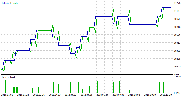
Despite the profits shown by the EA during the test, they are unlikely to remain in real trading. The futility of trading ordinary gaps on the examined symbols seems obvious. Such gaps are very rare (and become more rare with time) and small in size. The more in-depth consideration of the gaps generalization − price changes between trading sessions − seems more promising. Also, it makes sense to pay attention to the assets where ordinary gaps are more common.
Conclusion
Probabilistic methods are quite suitable for developing and configuring EAs. At the same time, they are in no way contrary to other possible methods. Instead, they often make it possible to supplement or rethink them.
In this article, we haven not touched on the topic of the general EA optimization by its parameters mentioning it only in passing. There is a significant connection between this area and the probabilistic approach (the theory of statistical solutions). Perhaps, I will study this question in detail later.
Attached files
Below you can find two EAs used for collecting statistics and one EA used for test trading.
| # | Name | Type | Description |
|---|---|---|---|
| 1 | gaps_reg_stat.mq5 | EA | Collecting gap statistics between consecutive ticks |
| 2 | gaps_ses_stat.mq5 | EA | Collecting gap statistics between sessions |
| 3 | gaps_ses_test.mq5 | EA | Test trading using gaps between sessions |